Welcome to Geo-Surface Drain Pro
Professional agricultural drainage design and terrain analysis
Geo-Surface Drain Pro is a comprehensive web-based platform for designing subsurface agricultural drainage systems. It combines high-resolution LiDAR elevation data with intelligent design tools to help agricultural consultants and professionals create optimal drainage layouts.

Key Capabilities
- High-Resolution Terrain Data: Access LiDAR elevation data with sub-meter accuracy across Canada and USA
- Click-to-View Elevation: Instantly check elevation at any point on the map with instant lookup from loaded DEM or auto-fetch from government servers
- Virtual Survey Tools: Draw drainage lines and see real-time elevation profiles
- Intelligent Design: Automated grade analysis and best-fit algorithms
- Advanced Analysis: Flow direction, wetness index, depressions, and ponding prediction
- Professional Output: Generate detailed PDF reports and georeferenced exports
- 3D Visualization: View terrain in immersive 3D with Cesium.js
Geo-Surface Drain Pro is available in two versions designed for different professional workflows:
| Feature Category | Drain Pro | Lite (Viewer) |
|---|---|---|
| PROJECT MANAGEMENT | ||
| Open & View Design Projects | ✓ | ✓ |
| Create New Projects | ✓ | ✗ |
| Save & Backup Project Files | ✓ | ✗ |
| Share Projects with Clients | ✓ | ✓ (view only) |
| DESIGN & DRAWING TOOLS | ||
| Draw Drainage Lines (Manual & GPS) | ✓ | ✗ |
| GPS Field Survey Integration | ✓ | ✗ |
| Edit & Modify Lines (Trim/Extend/Offset) | ✓ | ✗ |
| Delete & Reorganize Designs | ✓ | ✗ |
| Create Drainage Hierarchy (Mains/Secondaries) | ✓ | ✗ |
| ELEVATION & TERRAIN DATA | ||
| View Elevation Profiles | ✓ | ✓ (from restored backup) |
| Define Project Boundaries (Draw AOI) | ✓ | ✓ |
| Fetch High-Resolution LiDAR Data | ✓ | ✓ |
| Import Custom GeoTIFF DEMs | ✓ | ✓ |
| Click-to-View Elevation Anywhere | ✓ | ✓ |
| 3D Terrain Viewer (Cesium) | ✓ | ✓ |
| INTELLIGENT ANALYSIS | ||
| Generate Analysis Layers (TauDEM Processing) | ✓ | ✗ |
| Flow Direction & Accumulation Maps | ✓ | ✓ (view only) |
| Topographic Wetness Index (TWI) | ✓ | ✓ (view only) |
| Ponding Prediction & Depression Mapping | ✓ | ✓ (view only) |
| Automated Best-Fit Grade Calculation | ✓ | ✗ |
| Connection Validation & Enforcement | ✓ | ✗ |
| Depth Violation Detection | ✓ | ✗ |
| HYDRAULIC CALCULATIONS | ||
| Set Design Parameters (Grade/Depth/Diameter) | ✓ | ✗ |
| Automatic Pipe Sizing (Flow-Based) | ✓ | ✗ |
| Flow Rate Calculations | ✓ | ✗ |
| Drainage Coefficient Input | ✓ | ✗ |
| Material Quantity Estimates | ✓ | ✗ |
| Cost Projections | ✓ | ✗ |
| PROFESSIONAL EXPORTS | ||
| PDF Reports (Materials/Flow/Costs) | ✓ | ✗ |
| Ditch Assist Export (Machine Control) | ✓ | ✓ |
| KML Export (Google Earth) | ✓ | ✗ |
| CSV Design Data Export | ✓ | ✗ |
| Georeferenced Map Images (.jpg + .jgw) | ✓ | ✗ |
| PDF Map Export | ✓ | ✓ |
| High-Resolution Snapshots (.jpg) | ✓ | ✓ |
Drain Pro Version: Full-featured design suite for agricultural drainage consultants and professionals. Create designs from scratch, run advanced analysis, generate professional documentation, and share completed projects with clients.
Lite Version: Perfect for farmers, landowners, and stakeholders who need to review and understand drainage designs created by professionals. Open project backups shared by consultants, explore designs interactively, view elevation profiles and analysis layers, and export reference materials for field use.
Typical Workflow: Drainage consultant uses Drain Pro to design the system, generate analysis layers, validate connections, size pipes, and create professional PDF reports. The consultant then shares the project backup file with the client, who opens it in Lite to review the design, explore terrain analysis, view 3D visualizations, and export Ditch Assist files for their contractor.
Key Benefit: Clients can fully understand and interact with the design without needing expensive professional software or risk accidentally modifying the consultant's work.
Browser Requirements
- Modern web browser (Chrome, Firefox, Safari, or Edge recommended)
- JavaScript enabled
- Stable internet connection
- Minimum resolution: 1280x720 (1920x1080 recommended)
Optimal Performance
- Desktop or laptop computer (tablets supported but not optimal)
- 4GB RAM minimum, 8GB+ recommended
- Stable internet connection for LiDAR data downloads and analysis
- Chrome browser on Windows/Mac (recommended)
Performance automatically scales with project area. Larger regions download at lower resolution to maintain consistent performance. Use Chrome on desktop for best experience. Mobile devices work but have limited screen space for complex designs.
Interface Overview
Understanding the Geo-Surface Drain Pro workspace
The Geo-Surface Drain Pro interface is designed for efficient drainage design workflow with everything accessible from a single screen.

The left sidebar organizes your workflow into 3 main tabs:
1. Setup Tab (3-Step Workflow):
- Step 1 - Define Project Area: Upload a shapefile/KML boundary or draw manually on the map
- Step 2 - Get Elevation Data: Auto-fetch LiDAR from HRDEM (Canada) or 3DEP (USA), or upload your own GeoTIFF
- Step 3 - Generate Analysis Layers: Create flow direction, TWI, depressions, and ponding layers via TauDEM processing
2. Design Tab (Drainage Layout):
- Virtual Survey Tools: Draw lines, GPS survey, copy/offset, trim, extend, delete tools
- Design Parameters: Set grades, depths, pipe sizes, drainage coefficients for selected lines
- Grade Analysis: View profile charts, run Best Fit optimization, analyze line statistics
- Tile Sizing: Calculate required pipe sizes based on flow and contributing area
- Best Practices: Design guidelines and recommendations
3. Import/Export Tab (Data Management):
- Project Backup: Save/restore complete project files with all data
- Quick Exports: Save snapshot, Export PDF Map, Ditch Assist image, Export Map → KMZ
- Professional Reports: Generate comprehensive PDF reports with materials, flow, costs
- Design Data: Export design to Shapefile or KML for field implementation
- Analysis Data: Export/import flow analysis KML files
- Raw Data: Download LiDAR elevation GeoTIFF (EPSG:3857)
Click tab buttons at the top of the sidebar to switch between workflows.
The central map displays your project with multiple visualization options:
- Satellite imagery from Esri
- Elevation colorization (after fetching LiDAR)
- Hillshade visualization for terrain interpretation
- Analysis layers overlays
- Drawn drainage lines with labels
- Reference layers (contours, parcels, waterways)
The profile chart at the bottom shows elevation data for selected drainage lines:
- Blue line: Ground elevation profile along the drainage path
- Red line: Design grade showing proposed drain elevation and depth
- Green line: Minimum depth constraint line
- Magenta line: Maximum depth constraint line
Hover over the chart to see exact values. Toggle the chart on/off with the button in the bottom-right corner.
The floating toolbar in the Design tab provides quick access to line modification tools:
- Draw: Create new drainage lines
- Virtual Survey: Live profile while drawing
- Trim: Shorten lines to connection points
- Extend: Lengthen lines to connection points
- Offset: Create parallel laterals
- Delete: Remove individual lines
- Select to Delete: Remove multiple lines via polygon selection
- Clear All: Remove all drainage lines
Click the layers button (top-right of map) for quick access to common layer controls:
- Base layer selection
- Hillshade toggle
- Contour interval selection
- Flow direction overlay
- Reference layers (parcels, waterways)
A floating button on the map provides access to the 3D terrain viewer when elevation data is loaded:
- Availability: Button appears after DEM is successfully loaded
- Visualization: View terrain in perspective with drainage lines overlaid
- Navigation: Rotate (Ctrl + drag), pan (Shift + drag), zoom, and tilt the view
- Vertical Exaggeration: Adjust terrain relief for better visualization of subtle slopes
See the 3D Terrain Viewer section for detailed usage instructions.
Define Project Area
Step 1: Establish your field boundary or AOI
Every project begins by defining your field boundary or Area of Interest (AOI). This boundary:
- Determines the area for LiDAR data download
- Clips all visualizations to your project area
- Sets the working extent for terrain analysis
- Appears as a blue polygon on the map
If you have an existing boundary file from GIS software, surveying equipment, or farm management tools:

Steps:
- Click "Upload Field Boundary" in Setup tab, Step 1
- Select your file (or drag and drop)
- Wait for processing (usually 1-2 seconds)
- Verify the boundary appears on the map
Supported Formats:
- Shapefile: ZIP file containing .shp, .shx, .dbf, and .prj files
- KML/KMZ: From Google Earth, AgLeader, John Deere Operations Center, etc.
Critical: Boundary files MUST be in WGS84 (EPSG:4326) coordinates - Latitude/Longitude format. If your shapefile is in a projected coordinate system (UTM, State Plane, etc.), reproject it before upload using QGIS or ArcGIS.
If you don't have a boundary file, draw one directly on the map:

Steps:
- Use Location Search to navigate to your field
- Zoom in until field boundaries are clearly visible in satellite imagery
- Click "Draw Field Boundary" button
- Click around the field perimeter to place points
- Each click places a vertex
- Place points at corners and along curves
- Double-click to complete (or ESC to cancel)
- Zoom in close for accuracy
- Use satellite imagery to identify field edges and fence lines
- The boundary doesn't need to be perfect - you can always redraw
- Don't over-detail - simple polygons work fine
Projects can range from small fields to large regions:
- Maximum: 1,000,000 acres per project
- Resolution Trade-off: Larger regions automatically download at lower resolution to maintain performance. This is by design - performance stays consistent regardless of area.
- Detail Level: Choose project size based on your analysis needs, not performance concerns
Get Elevation Data
Step 2: Fetch high-resolution LiDAR terrain data
After defining your boundary, fetch high-resolution elevation data that forms the foundation for drainage design and terrain analysis.
Data Sources:
- Canada: HRDEM (High Resolution LiDAR) at 1-2 meter resolution from Natural Resources Canada
- USA: 3DEP (3D Elevation Program) from USGS at 1-10 meter resolution depending on location
In areas without high-resolution LiDAR coverage, a coarser MRDEM (Medium Resolution 20-30m) base layer may be available through the Layers popup as a grayscale overlay option. However, this lower resolution data cannot be used for drainage design or analysis layer generation.

Download Times:
Typical download time is 10-30 seconds for most fields. The system uses optimized resolution settings to ensure fast downloads regardless of field size.
The system fetches raw elevation data (GeoTIFF format) and processes it locally in your browser to create the HD Elevation layer, which combines both colorization and hillshade into a single visualization. All data is clipped to your project boundary.
Elevation data is fetched from government servers (Natural Resources Canada and USGS). During peak hours, these servers can become overloaded, which may cause download failures or timeouts.
This is not a Geo-Surface issue - these are external government infrastructure limitations beyond our control. Typically, servers recover within a few minutes, but occasionally outages can last longer. If a download fails, please wait a few minutes and try again.
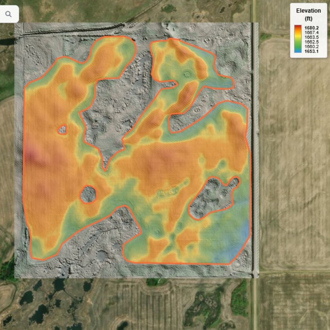
After fetching, the HD Elevation layer appears on your map, combining elevation colorization with hillshade relief for comprehensive terrain visualization.
Elevation Color Ramps:
Choose from 17 different color schemes to visualize elevation data. Access the color ramp selector in the Layers popover under the Elevation Data section.
Available color ramps include:
- Spectral (default): Purple → Blue → Green → Yellow for intuitive low-to-high visualization
- Classic: Blue → Green → Yellow → Red traditional elevation colors
- Plasma/Inferno/Magma: Scientific color schemes with excellent contrast
- Electric/Neon: High-visibility vibrant colors for presentations
- Terrain: Earth tones mimicking natural topographic maps
- Rainbow/Turbo: Full spectrum for maximum differentiation
All color ramps use quantile-based mapping that adapts to your field's elevation range, ensuring useful color variation even on flat terrain. Your selection is remembered between sessions.
Hillshade Relief:
3D-style shaded relief is automatically combined with the color gradient, simulating northwest sunlight to emphasize:
- Topographic features and landforms
- Subtle elevation changes and micro-topography
- Ridges, valleys, and drainage pathways
Toggle the HD Elevation layer on/off using the floating Layers button (layer stack icon) on the map. The layer combines both colorization and hillshade as a unified visualization.
If LiDAR Fetch Fails:
- Verify Location: Ensure boundary is in correct region (Canada vs USA)
- Check Coverage: Enable LiDAR Coverage layer to see areas where high-resolution LiDAR is available. Only areas showing LiDAR coverage can be fetched - coarse terrain areas cannot be downloaded.
- Try Again: Servers occasionally timeout - retry after a few minutes
- Alternative: Use Custom DEM Upload feature if you have elevation data from other sources
LiDAR coverage is extensive but not universal. High-resolution data is available for most agricultural regions, but some remote areas may only have coarser resolution or no coverage.
If you have your own elevation data from alternative sources (professional surveys, RTK drone mapping, other LiDAR sources, etc.), you can import a custom GeoTIFF file instead of fetching from public servers.
- Higher accuracy: Professional RTK surveys provide centimeter-level accuracy vs. LiDAR's 10-30cm vertical accuracy
- Recent data: Your field may have changed since LiDAR was captured (grading, earthwork, etc.)
- Coverage gaps: LiDAR not available in your location
- Alternative sources: Access to commercial LiDAR or other high-quality elevation data
GeoTIFF Requirements:
How to Prepare Your GeoTIFF:
Most elevation data is provided in a geographic coordinate system (like WGS84 / EPSG:4326) or a local projected system (like UTM zones). You must reproject to EPSG:3857 before importing.
Using QGIS to Prepare Your GeoTIFF:
QGIS is a free, open-source GIS application perfect for preparing elevation data. Download QGIS
- Load your elevation file:
- Open QGIS
- Drag and drop your elevation GeoTIFF into QGIS
- Or use: Layer → Add Layer → Add Raster Layer
- Check current coordinate system:
- Right-click the layer in the Layers panel
- Select Properties → Information
- Note the current CRS (Coordinate Reference System)
- Reproject the raster:
- Go to: Raster → Projections → Warp (Reproject)
- Source CRS: Should auto-detect (verify it's correct)
- Target CRS: Type "3857" in the search box and select "EPSG:3857 - WGS 84 / Pseudo-Mercator"
- Resampling method: Select "Bilinear" (good balance) or "Cubic" (smoother, slower)
- NoData value: Enter -9999 (or leave as default if your data uses standard values)
- Output file: Click [...] and choose where to save (e.g., "my_field_3857.tif")
- Click Run
- Verify the result:
- The reprojected layer will be added to your map
- Right-click → Properties → Information
- Confirm CRS shows "EPSG:3857"
- Check that extent coordinates are large numbers (millions), not lat/lon decimals
If you're comfortable with command-line tools, you can use GDAL directly:
gdalwarp -s_srs EPSG:4326 -t_srs EPSG:3857 \
  -r bilinear -dstnodata -9999 \
  input.tif output_3857.tif
Parameters explained:
-s_srs EPSG:4326- Source coordinate system (replace 4326 with your source EPSG code)-t_srs EPSG:3857- Target coordinate system (Web Mercator)-r bilinear- Resampling method (bilinear is recommended)-dstnodata -9999- Set NoData value to -9999
Don't know your source EPSG code?
gdalinfo input.tif
Look for the "Coordinate System" section in the output.
Importing Your GeoTIFF into Geo-Surface:
- Define your boundary first (Step 1) - the system needs to know your project area
- In the Setup Workflow panel, look for the "Upload Custom DEM" button in Step 2
- Click the button and select your EPSG:3857 GeoTIFF file
- The system will:
- Validate and load the file
- Extract origin, resolution, and extent from metadata
- Create colorized and hillshade visualizations automatically
- Zoom the map to your elevation data extent
- Enable the "Create Drainage Layers" button for TauDEM processing
- You'll see "GeoTIFF loaded successfully" when complete
Once loaded, your custom GeoTIFF works exactly like LiDAR data - you can generate analysis layers, draw drainage designs, export profiles, and create reports. The data is also saved in project backups.
Common Issues and Solutions:
Likely causes:
- Wrong coordinate system: File is not in EPSG:3857. Reproject using QGIS or GDAL.
- Corrupted file: Try re-exporting from your source software
- Missing georeferencing: File lacks embedded coordinate system metadata
- Unsupported format: Must be standard GeoTIFF format
This indicates incorrect coordinate system. The file may be in a different projection or the metadata may be wrong.
Solution: Verify the source coordinate system and reproject to EPSG:3857 using the QGIS instructions above.
Your source data is in feet, but Geo-Surface expects meters.
Solution in QGIS:
- Open Raster Calculator: Raster → Raster Calculator
- Enter formula:
"your_layer@1" / 3.28084 - Save output, then reproject that result to EPSG:3857
Many drone pilots use Pix4D, DroneDeploy, or similar photogrammetry software to create DEMs. These typically export in the local coordinate system (often UTM). Export your DEM as GeoTIFF, note the coordinate system, then use QGIS to reproject to EPSG:3857 before importing to Geo-Surface.
If you have surveyed elevation points from professional field surveys (RTK GPS, total station, etc.), you can upload them as a point shapefile and the system will automatically interpolate a high-resolution DEM tailored to your field.
- Professional surveys: You have RTK GPS or total station survey points with precise elevations
- Maximum accuracy: Survey-grade points provide centimeter-level accuracy far exceeding LiDAR
- Recent field changes: Your field has been modified since LiDAR was captured (grading, land leveling, etc.)
- LiDAR gaps: High-resolution LiDAR data not available in your area
- Custom coverage: Generate a DEM perfectly tailored to your specific survey points and field boundary
Point Shapefile Requirements:
Important: Elevation points upload requires a shapefile boundary (uploaded in Step 1). If you drew your boundary manually or uploaded KML/KMZ, you must replace it with a shapefile boundary before using this feature.
How It Works:
- Upload shapefile boundary (Step 1 - Setup Workflow)
- Must be a zipped shapefile (not KML/KMZ)
- Must contain your field/project boundary as polygon(s)
- Must be in WGS84 (EPSG:4326) coordinate system
- Click "Upload Elevation Points" button (Step 2)
- Button becomes enabled after shapefile boundary is uploaded
- Select your zipped point shapefile
- Select elevation column and units
- System automatically detects all numeric fields in the shapefile
- Choose which field contains elevation values
- Specify units: Feet or Meters
- Review sample value to verify correct column and units
- Server-side interpolation processing
- Files are uploaded to Geo-Surface processing server
- Points are validated and reprojected to Web Mercator
- Advanced interpolation creates smooth elevation surface from your points
- DEM is clipped precisely to your boundary
- Processing typically takes 2-5 minutes depending on point density
- Automatic DEM loading
- Interpolated DEM is automatically downloaded and loaded
- Colorized and hillshade visualizations are generated
- Map zooms to your data extent
- DEM manager status updates to show successful load
- Ready to generate analysis layers (Step 3)
Preparing Your Survey Points in QGIS:
If your survey points are in CSV or text format, use QGIS to convert them to a shapefile:
- Load CSV file:
- Open QGIS
- Layer → Add Layer → Add Delimited Text Layer
- Select your CSV file
- Choose correct delimiter (comma, tab, etc.)
- X field: Select your longitude column
- Y field: Select your latitude column
- Geometry CRS: Select EPSG:4326 (WGS84)
- Click Add
- Verify elevation field is numeric:
- Right-click layer → Open Attribute Table
- Check that elevation values appear as numbers (not text)
- If showing as text, you may need to clean your CSV file
- Export as shapefile:
- Right-click the layer → Export → Save Features As
- Format: ESRI Shapefile
- File name: Choose location and name (e.g., "survey_points.shp")
- CRS: EPSG:4326 - WGS 84
- Click OK
- Zip all shapefile components:
- Navigate to the folder where you saved the shapefile
- Select all related files: .shp, .shx, .dbf, .prj (and .cpg if present)
- Create a ZIP archive containing these files
- This ZIP file is what you'll upload to Geo-Surface
If your survey points are in a different coordinate system (e.g., UTM, State Plane), reproject to WGS84 (EPSG:4326):
- Load your points: Drag and drop your shapefile into QGIS
- Check current CRS: Right-click layer → Properties → Information → CRS
- Reproject:
- Right-click layer → Export → Save Features As
- Format: ESRI Shapefile
- CRS: Type "4326" and select "EPSG:4326 - WGS 84"
- File name: Save as new file (e.g., "survey_points_wgs84.shp")
- Click OK
- Verify result:
- The new layer should load in QGIS
- Check Properties → Information → CRS shows EPSG:4326
- Coordinates should be decimal degrees (e.g., -95.5, 42.3)
- Zip and upload: Zip all components and upload to Geo-Surface
Once the interpolated DEM is loaded, it works exactly like LiDAR or custom GeoTIFF data - you can generate analysis layers (Step 3), draw drainage designs, export profiles, and create reports. The DEM is also saved in project backups for future use.
Interpolation Details:
The server uses advanced Radial Basis Function (RBF) interpolation to create a smooth elevation surface from your survey points. The algorithm:
- Honors exact elevations at each survey point location
- Creates smooth transitions between points using thin-plate spline method
- Applies Gaussian smoothing (σ=7.5 meters) to reduce noise and artifacts
- Produces a continuous elevation surface clipped precisely to your boundary
- Outputs DEM in EPSG:3857 (Web Mercator) with meters as vertical units
Common Issues and Solutions:
Cause: You either haven't uploaded a boundary, or you uploaded KML/KMZ or drew the boundary manually.
Solution:
- Go to Step 1 and upload a shapefile boundary (zipped .shp, .shx, .dbf files)
- The boundary must be in WGS84 (EPSG:4326) coordinate system
- KML/KMZ boundaries and manually drawn boundaries are not compatible with elevation points upload
Cause: The shapefile doesn't contain any numeric elevation fields, or the field type is set to text/string.
Solution:
- Open the shapefile in QGIS and check the attribute table
- Ensure you have a field containing numeric elevation values
- If elevation values appear as text, create a new numeric field and copy values using Field Calculator
- Re-export as shapefile and try again
Cause: Your point shapefile is in a different coordinate system (e.g., UTM, State Plane).
Solution: Use QGIS to reproject your points to WGS84 (see accordion above for step-by-step instructions).
Cause: Interpolation is taking longer than expected, possibly due to very large point datasets or server load.
Solution:
- For very large point datasets (>50,000 points), consider decimating or filtering to a representative sample
- Try again during off-peak hours
- Contact support if the issue persists - there may be a server issue
- Minimum coverage: Ensure points distributed across entire field area
- Optimal spacing: 30-60 feet (10-20 meters) between points for best results
- Capture terrain features: Include extra points on ridges, swales, and drainage ways
- Boundary points: Survey points along field perimeter help ensure accurate edge interpolation
- Quality over quantity: 200-500 well-distributed RTK points typically better than 5,000 poorly distributed points
Click to View Elevation
Click anywhere on the map to instantly view elevation data at that location - a quick way to check elevations without loading a full DEM.
How It Works:
- With Loaded DEM: Instant elevation lookup from your loaded elevation data (Step 2)
- Without Loaded DEM: Automatically fetches elevation from government servers:
- Canada: HRDEM (LiDAR) or MRDEM (medium resolution) depending on location
- USA: 3DEP elevation service
Elevation Popup:
The popup shows:
- Elevation in feet
- Data source (in Canada: "Local DEM", "HRDEM", or "MRDEM")
Use this feature for quick spot checks of elevation across your field, verifying outlet elevations, or comparing elevations between locations. In MRDEM areas, elevation data is available but should be used with caution due to lower resolution (20-30m).
Analysis Layers
Step 3: Generate advanced terrain analysis (Drain Pro only)
After fetching elevation data, Drain Pro users can generate advanced terrain analysis layers using TauDEM algorithms running on a dedicated processing server.
Analysis layer generation is available only in Geo-Surface Drain Pro. Lite users can view analysis layers if included in project files shared by Drain Pro users.
Processing Time:
Processing time is generally under 1 minute for most projects. Very large regions may take slightly longer, but due to automatic resolution optimization for larger areas, processing times remain consistent.
Analysis processing uses a shared queue system. During busy periods, you may see your position in the queue (e.g., "Position in queue: 2"). Jobs are processed sequentially, typically taking 30-60 seconds each once they start.
Note: You cannot work in the application while processing is in progress. Wait for the layers to complete before continuing your workflow.
- Complete Steps 1 and 2 (Define Boundary, Fetch Elevation Data)
- In Step 3, click "Create Drainage Layers"
- Progress indicator shows processing stages
- When complete, new layers are available via the floating Layers button on the map

Processing Stages:
- Major Flow Paths: Surface flow analysis based on fill & spill modelling
- Wetness Potential Index: Areas prone to saturation and wetness
- Ponding Risk: Areas where standing water is likely to accumulate
- Depressions: Closed depressions and low areas in the terrain
Surface flow paths based on fill & spill modelling that shows how water actually moves across the terrain when depressions fill and overflow.
Use for:
- Identifying natural drainage patterns
- Locating flow convergence areas (where water concentrates)
- Planning optimal main drain routes (follow natural flow)
- Understanding how water moves across the field

Toggle on/off via the floating Layers button under "Analysis Layers"
Identifies areas prone to saturation and wetness based on terrain characteristics.
- Tan/Yellow: Dry, well-drained areas (low wetness potential)
- Green: Moderate wetness potential
- Cyan: Elevated wetness potential
- Blue: High wetness potential - prioritize for drainage
The color gradient runs from Tan→Yellow→Green→Cyan→Blue (Dry→Wet).
Design Applications:
- Prioritize drainage in high wetness potential areas
- Use closer lateral spacing in problem zones
- Wider spacing acceptable in well-drained areas
- Combine with field observations for validation

Identifies closed depressions (low spots surrounded by higher ground) where water naturally accumulates.
- Grayscale overlay: White areas show deeper depressions, dark gray/black shows shallow or no depression
- Intensity: Brighter (whiter) areas indicate deeper depressions
Use for:
- Locating potential standing water areas
- Planning outlet locations
- Identifying areas needing surface drainage
- Understanding natural water accumulation patterns

Identifies areas at risk of ponding based on depression depth, surrounding slope, and flow patterns.
Interactive Risk Slider: Adjust the threshold to visualize areas at different levels of ponding risk. Higher slider values show only the most severe problem areas, while lower values reveal broader areas of concern.
Applications:
- Identify areas most at risk for standing water
- Visualize ponding risk severity across the field
- Prioritize drainage investment in high-risk zones
- Communicate drainage needs to clients visually
The slider adjusts the sensitivity threshold for highlighting ponding risk areas. Lower values show more area (including moderate risk), while higher values focus only on severe problem spots. This is a relative risk indicator, not an absolute water depth measurement.

Analysis layers should be used for ALL drainage design projects. They provide critical intelligence that significantly improves design quality and return on investment:
Key Benefits:
- Natural Flow Paths: Understand how water actually moves across the field. Both surface drainage and tile drainage are more effective when they follow natural flow patterns rather than fighting them.
- Optimal Outlet Placement: Identify the best locations for outlets based on natural drainage convergence and flow accumulation.
- Target High-Risk Wet Areas: Focus drainage investment on areas with the highest wetness potential and greatest yield impact.
- Maximize ROI: Design efficient systems that address actual problem areas rather than guessing, reducing over-drainage and under-drainage.
- Better Main Placement: Route main drains along natural flow paths for maximum effectiveness and proper sizing.
Analysis layers take less than 1 minute to generate and can save hours of design time while dramatically improving system performance. Use them on every project - even fields you know well can reveal drainage patterns that aren't obvious from elevation alone.
Reference Layer Overlays
Import and georeference custom image and vector layers
Reference layers allow you to overlay custom images and vector data onto your project map. These can be scanned maps, photos, screenshots, KML files, or shapefiles that provide additional context for your drainage design.
Common Use Cases:
- Prior Designs: Overlay existing drainage maps to reference past installations
- Utility Locations: Import utility maps showing buried cables, pipelines, or water lines
- Soil Maps: Layer EC maps, soil survey data, or yield maps for reference
- Field Photos: Georeference aerial photos or drone imagery from other sources
- Planning Documents: Import survey drawings, engineer plans, or CAD exports
- Property Boundaries: Load parcel boundaries, easements, or legal descriptions
Reference layers are visual aids only. Accuracy of georeferenced or imported layers cannot be guaranteed and depends on source data quality and georeferencing precision. For critical infrastructure like utilities, always obtain professional locates and perform field verification before excavation. Reference layers assist with planning but do not replace proper surveying, testing, or locate services.
Raster Image Formats:
- JPG/JPEG: Photos, scanned maps, screenshots (manual georeferencing)
- PNG: Graphics, screenshots, exported maps (manual georeferencing)
- BMP: Windows bitmap images (manual georeferencing)
- GeoTIFF: Georeferenced images with embedded coordinate data (auto-placed)
JPG, PNG, and BMP images require 4-point manual georeferencing to position and orient them on the map. GeoTIFF files are placed automatically using their embedded coordinate metadata — no manual georeferencing needed.
Vector Data Formats (auto-loaded, no georeferencing needed):
- KML: Google Earth files with points, lines, or polygons
- KMZ: Compressed KML files
- Shapefile (ZIP): Zipped folder containing .shp, .dbf, .shx files
Vector formats are assumed to be in WGS84 (EPSG:4326) coordinate system and are automatically transformed to the map projection.
If your data is already georeferenced (KML, KMZ, Shapefile), use those formats - they load instantly. If you only have a scanned map or photo, use the manual georeferencing workflow described below.
- Locate the folder icon floating button at the bottom-left of the map labeled "Load Reference Data"
- Click to open the Load Reference Data modal
- Upload your file via drag-and-drop or the Browse button
The tool automatically detects file type and routes to the appropriate loader:
- GeoTIFF (.tif): Auto-placed on the map at the correct position using embedded georeferencing
- Other raster images (.jpg, .png, .bmp): Opens the manual georeferencing workflow
- Vector data (.kml, .kmz, .zip): Loads immediately and zooms to features
GeoTIFF files contain embedded coordinate metadata that allows the application to automatically place them at the correct position on the map — no manual georeferencing required.
How It Works:
- Click Load Reference Data
- Upload a .tif or .tiff file
- The image is parsed, georeferenced, and placed on the map automatically
- The map zooms to fit the image extent
Supported Image Types:
- RGB / RGBA: Color images (aerial photos, satellite imagery, scanned maps)
- Single-band (grayscale): Automatically rendered with min/max contrast stretch
Supported Coordinate Systems:
- EPSG:4326 (WGS84 — latitude/longitude)
- EPSG:3857 (Web Mercator)
- UTM zones and other projected coordinate systems (automatic reprojection)
When you upload a JPG, PNG, or BMP image, the georeferencing interface opens with split-view panels: your image on the left, a map preview on the right.
Step-by-Step Georeferencing:
-
Click 4 Reference Points on the Image
Click identifiable features in the image such as:
- Field corners or property corners
- Road intersections
- Building corners
- Fence posts or utility poles
- Any clearly visible landmark
Important: Points do NOT need to be at the image corners. For scanned maps with white borders, click interior features on the actual map content. The system uses affine transformation to handle rotation and scaling.
-
Click the Same Locations on the Map
For each point you clicked on the image, click the same real-world location on the map preview. The map starts centered on your current project area.
As you place points, numbered markers (1, 2, 3, 4) appear showing your selections.
-
Preview the Placement
After placing all 4 point pairs, the system:
- Calculates the affine transformation (rotation, scale, translation, shear)
- Pre-renders the transformed image with proper rotation
- Displays a preview overlay on the map
Review the placement. If the alignment isn't correct, click Reset Points and try again with different reference points.
-
Add to Map
Once satisfied with the preview, click Add to Map. The georeferenced image is added to your project as a semi-transparent overlay (85% opacity).
Unlike traditional corner-only georeferencing, this tool supports clicking reference points anywhere within the image. This is ideal for paper maps with white borders or maps where north isn't at the top. The affine transformation automatically handles rotation and ensures the image aligns correctly based on your chosen reference points.
The georeferencing system fully supports rotated images. If your scanned map has north pointing to the side or at an angle, simply select your reference points and the system will automatically calculate the required rotation, scaling, and positioning to align it correctly on the map.
Tips for Best Results:
- Spread Points Out: Choose reference points spread across the entire image area, not clustered in one corner
- Use Precise Features: Sharp corners and intersections work better than vague features
- Zoom In: Pan and zoom the map preview to click reference locations as precisely as possible
- Avoid Collinear Points: Don't place all 4 points in a straight line - use 3+ corners of a polygon
- Check Scale: After georeferencing, verify distances roughly match reality using the map's scale
Vector data loads instantly without manual georeferencing. The system:
- Reads the vector features from the file
- Transforms coordinates from WGS84 (EPSG:4326) to the map projection (EPSG:3857)
- Creates a new vector layer with appropriate styling
- Zooms the map to fit all features
- Adds the layer to the Map Layers control
Shapefile Requirements:
When uploading shapefiles, ensure your ZIP file contains at minimum:
- .shp: Main geometry file (required)
- .dbf: Attribute data file (optional but recommended)
- .shx: Shape index file (optional)
The shapefile parser supports:
- Polygons: Including multi-part polygons with holes
- Polylines: Lines and multi-line features
- Points: Single point features
All vector imports assume WGS84 (EPSG:4326) geographic coordinates (longitude/latitude). Most KML files and modern shapefiles use this standard. If your shapefile is in a different projection, reproject it to WGS84 using QGIS or ArcGIS before importing.
KML/KMZ Features:
KML imports preserve:
- Styles: Line colors, fill colors, widths
- Names: Feature labels and descriptions
- Multiple Features: All points, lines, and polygons in the file
Toggle Visibility:
- Click the Layers button (floating button on map)
- Scroll to the Reference Layers section
- Toggle the eye icon to show/hide individual reference layers
Delete Reference Layers:
- Open the Layers popover
- Locate the reference layer in the Reference Layers section
- Click the trash icon next to the layer name
- Confirm deletion when prompted
All reference layers appear in the Layers control with their file name displayed for easy identification.
Raster reference images are displayed at 85% opacity by default, allowing you to see both the reference layer and the base imagery beneath. Vector layers are drawn with semi-transparent fills for better visibility.
Multiple Reference Layers:
You can load multiple reference layers simultaneously. For example:
- Utility map as a georeferenced image
- Property boundary as a shapefile
- Prior drainage design as a KML file
Each layer can be toggled independently for different planning views.
Reference layers are automatically included in project backups created via the Import/Export tab.
What's Saved:
- Raster Images: Converted to PNG format and stored in the backup ZIP
- Georeferencing Data: Extent, transformation, opacity settings
- Vector Data: Exported as GeoJSON in WGS84 coordinates
- Layer Names: Original file names preserved
Restore Behavior:
When you restore a project backup:
- All reference layers are automatically recreated
- Georeferenced images are positioned exactly as they were
- Vector layers are re-imported with original styling
- Layers appear in the Map Layers control ready to toggle
Reference layers make your project backups fully self-contained. When sharing project files with clients or colleagues, all reference data travels with the backup - no need to separately share image files or KML files.
Delete the layer, reload the image, and try again with different reference points:
- Choose reference points that are more spread out
- Use sharper features (corners, intersections) rather than vague features
- Zoom in more on the map when clicking reference points
- Ensure your reference points aren't all in a straight line
Remember: Accuracy depends on the quality of your source image and how precisely you click reference points. Sub-meter accuracy is challenging with manual georeferencing.
Yes! The georeferencing system fully supports rotation. Simply select your 4 reference points and the system automatically calculates the required rotation angle. The pre-rendered image will be rotated to align correctly with the map.
Check these common issues:
- Missing .shp file: ZIP must contain at minimum a .shp file
- Wrong projection: Shapefile must be in WGS84 (EPSG:4326). Use QGIS to reproject if needed
- Corrupt file: Try opening in QGIS first to verify integrity
- Unsupported geometry: Very complex geometries or multipart features may not parse correctly
Currently, opacity is fixed at 85% for raster images. This provides a good balance between visibility of the reference layer and the base imagery beneath. Future versions may add opacity controls.
Yes. The tool clears all memory when you delete a reference layer and resets the file input, allowing you to immediately re-upload the same file. This is useful for re-georeferencing an image with better reference points.
Reference layers appear in:
- Screenshot/Map Image Exports: Yes, if layer is visible when you capture
- Project Backups: Yes, always included
- KML/CSV Design Exports: No, only drainage lines are exported
- PDF Reports: No, only drainage design and statistics
To export reference layers separately, use the Map Image export tool with the layer visible, or save the project backup and extract the reference files from the ZIP.
- Source Quality Matters: High-resolution scans produce better georeferencing results than blurry photos
- Use Vector When Possible: If you have the choice between a scanned map and a KML/shapefile of the same data, use the vector format - it's more accurate
- Test Alignment: After georeferencing, draw a test line over a known feature and compare with satellite imagery to verify accuracy
- Document Limitations: When sharing designs that relied on reference layers for utility placement, include disclaimers about accuracy and need for professional locates
- Layer Organization: Use descriptive file names before upload (e.g., "2015_tile_map.jpg" instead of "IMG_1234.jpg")
- Backup Regularly: Reference layers are included in project backups, so save backups after adding reference data
- Legal/Survey Data: For official boundary data, use certified survey files in shapefile format rather than georeferencing scanned documents
Video Tutorials
Step-by-step video guides to master Geo-Surface Drain Pro
Learn how to use Geo-Surface Drain Pro through our comprehensive video tutorial library. Click any video below to watch.
Geo-Surface Introduction
Get familiar with the Geo-Surface interface, navigation controls, and core features. Learn how to navigate the map, access tools, and understand the tab-based workflow.
Getting Started: Setup Tab Workflow
Master the essential first steps: define your field boundary, fetch high-resolution LiDAR elevation data, and generate analysis layers including flow direction and ponding overlays.
Drainage Parameters Settings
Configure your drainage design defaults: set min/max depth limits, define minimum grades for surface and tile drainage, choose default pipe sizes and forms, and specify ditch bottom widths for earthwork calculations.
Drawing Proposed Drainage Routes
Draw tile and surface drainage routes directly on the map. See how Geo-Surface automatically fetches elevation profiles, connects tributaries to main runs, and builds a complete drainage hierarchy.
Design Validation Tools
Understand Geo-Surface's automatic validation system. Learn how each drain is checked for depth violations (staying within min/max limits) and connection violations (ensuring laterals connect above the main's install depth).
Understanding Best Fit and Manual Proposed Grades
Explore Geo-Surface's automatic best-fit grade calculation that simulates machine control systems in the field. Learn how to manually create simpler grade lines for scenarios like excavator-dug tile mains.
Creating Parallel Tile Laterals
Create multiple offset tile laterals at regular spacing to quickly design large-scale pattern tile layouts. Use the Break Line tool to dynamically adjust lateral lengths and target specific areas requiring drainage.
Line Editing Tools
Master the line editing toolkit: clip ends of single or multiple routes, extend lines to reach connections, and delete selected or all drainage features from your project.
Tile Sizing
Set pipe sizes and forms for tile drainage systems. Learn how to use the auto-sizing feature to automatically calculate optimal diameters for tile mains and sub-mains based on flow requirements.
Creating a Full Field Targeted Drainage Design
Complete walkthrough of designing a targeted drainage system from start to finish. Watch a real-world example tying together all the tools and workflows covered in previous tutorials.
Backing Up and Restoring Projects
Develop the habit of regularly backing up your projects and learn how to restore them to continue working. Pro users can share project backups with others to view in the free Geo-Surface Viewer.
Loading a Reference Image
Import any screenshot or scanned map, quickly geotag it, and add it as a map layer. Perfect for referencing paper maps showing utility locations, EC maps, soil maps, or other data while designing.
Export Options
Create professional drainage reports, map image exports, and high-resolution overlay exports. Learn how to load these exports into popular machine control systems to guide installation of your drainage plan.
Typical Workflow
Complete walkthrough for Drain Pro users: from field setup to final export
This guide walks you through a complete drainage design project from start to finish, following the workflow that most Drain Pro users will use. While individual sections of the manual provide detailed information on specific features, this workflow shows how everything connects together in a real project.
Start with small, simple projects to build confidence and understanding. As you gain experience, gradually tackle larger and more complex fields. The more you use the system, the better you'll understand its capabilities and limitations.
Option A: Import Field Boundary (Recommended)
If you have a shapefile of your field boundary, this is the best approach:
- Drag and drop the shapefile (.shp, .shx, .dbf, .prj files) onto the map
- The map will automatically zoom to your field location
- The boundary is precisely defined with no manual drawing required
Option B: Manual Boundary Drawing
If you don't have a shapefile:
- Search for your field location using the search tool
- Navigate to the field using the map controls
- Draw a boundary around your area of interest
When drawing manually, you can include additional areas that may not be in the official field boundary, such as the route to an adequate outlet (named waterbody, large drainage channel, etc.). This helps you plan the entire drainage system including outlet options.
When you fetch LiDAR data, the system automatically fetches for a slightly larger area than your boundary. LiDAR is also fetched for areas inside interior field boundaries (holes), allowing you to incorporate those areas into your designs if needed.
- Click the "Fetch LiDAR" button in the Setup Workflow panel
- Wait a few seconds for the data to download and process
- The colorized HD elevation layer will appear on your map
Occasionally, Canadian and US LiDAR servers experience high traffic. If your fetch doesn't complete on the first try, wait a minute or two and try again. These delays are typically brief, lasting only a few minutes while large requests are processed.
After successfully fetching LiDAR, create a project backup. Your elevation data is saved in the backup file, so in future sessions you can simply restore the backup rather than re-downloading from the servers.
Alternative: Custom GeoTIFF
If you have your own elevation data (surveyed DEM, alternative LiDAR source, etc.), you can import a custom GeoTIFF file instead of fetching from public servers. See the Get Elevation Data section for details.
Once you have elevation data loaded, generate the terrain analysis layers:
- Click "Create Drainage Layers" in the Setup Workflow panel
- Wait for TauDEM processing to complete (typically under 1 minute)
- The following layers will be generated:
- Major Flow Paths: Shows natural surface water movement
- Wetness Potential: Areas prone to saturation
- Ponding Risk: Where standing water accumulates
- Depressions: Closed low areas in the terrain
Analysis layers are also saved to project backups. Now is an excellent time to create a backup file with your boundary, elevation data, and analysis layers all preserved for future use.
Before drawing any drainage lines, take time to understand your field's natural drainage characteristics:
Examine the Flow Patterns
Toggle on the Major Flow Paths layer and study how water naturally moves across the field. These flow lines reveal:
- Natural drainage routes following the terrain's relief
- Convergence areas where flow concentrates
- Potential outlet locations
- Areas where water naturally accumulates
Drains that follow natural flow routes are easier to install and more effective. Trying to route drainage against natural flow typically results in: deep excavations, expensive earthwork, difficult installations, and less effective drainage performance.
Identify Priority Areas
Use the analysis overlays to target problem areas:
- Ponding overlay: Shows where standing water accumulates
- Wetness Potential: Identifies areas prone to saturation
- Depressions: Reveals low spots and potholes
Targeting high-risk areas identified by the analysis layers provides the biggest return on investment. Even pattern tile systems can be designed to prioritize problem areas while avoiding zones shown to have very low drainage risk, representing significant cost savings without compromising performance.
Additional Analysis Tools
Use these tools to deepen your understanding:
- Contour lines: Visualize elevation changes and slope
- 3D View: See terrain relief in three dimensions
- Colorized elevation: Quickly identify high and low areas
- Measure tool: Check distances and areas
Planning the Route
- Identify the outlet point: Ideally, follow a major flow line to its natural outlet, or at minimum use flow lines to guide placement
- Start at the outlet: Begin drawing from downstream moving upstream
- Follow logical terrain: Use the Draw Manual Survey tool and zoom in to follow natural contours
- Don't draw straight through ridges or hills when there's a route around them
- Follow valleys and low areas where possible
- Stay close to natural flow paths
Test Multiple Options
Don't settle on the first route you draw. Experiment with different paths and examine the elevation profiles to find the best option that:
- Validates without errors: No depth violations (red X marks)
- Stays within viable depth range: Not too deep for equipment, not too shallow to be effective
- Has a valid outlet: Starting depth is at or above the deepest possible outlet elevation
- Maintains appropriate grade: See grade targets below
Grade Targets
- Surface drains: Minimum 0.04-0.05% to keep water moving, but try to keep under 1% on unstable soils to minimize erosion risk
- Tile drains: Minimum 0.1%, preferably 0.2% or more (though 0.1% often necessary on flat fields)
- Maximum grade: Try to keep runs under 1-2% to avoid excessive velocity and potential issues
Finding viable routes often requires trial and error. Use the profile view to evaluate each attempt, adjust your route, and try again. There's rarely a perfect solution—the goal is finding the most practical compromise between depth, grade, and placement.
Once your main drain is placed, you can connect additional drainage lines depending on your system type:
Surface Drainage or Targeted Tile Systems
For systems targeting specific problem areas:
- Follow flow paths: Use the Major Flow Paths layer as your primary guide—it shows the natural path water takes from wet areas to potential outlets
- Target high-risk zones: Connect areas identified by ponding and depression layers to your main drain
- Expect challenges: While flow paths show the path of least resistance, you may still encounter ridges or elevation obstacles to navigate
- Size considerations:
- 50-100 feet wide wet areas: One or two perforated pipes may suffice
- Wider than 100 feet: Consider pattern tile instead
- Sloughs and potholes: May require surface intakes for faster water infiltration (soil infiltration alone may be too slow)
Pattern Tile Systems
For systematic lateral tile drainage:
- Draw the first lateral: Connect it to your main drain, ensuring it validates (green status)
- Use Offset Lines tool: Create exact copies at regular spacing (e.g., 50-foot centers)
- For best results, keep laterals straight
- Orient laterals at an angle that maintains valid depth and grade
- Set a breakline: Draw a line representing where laterals should end
- Use satellite imagery to avoid obstacles
- Reference elevation layers to stop before hills
- Use wetness/ponding data to optimize coverage
Pattern tile doesn't have to cover every inch uniformly. Use wetness and ponding potential to target high-risk areas more intensively while reducing or eliminating coverage in very low-risk zones. This can dramatically reduce costs without impacting drainage effectiveness.
As you draw drainage lines, the system automatically performs validation checks:
Depth Validation
The system runs a best-fit simulation on each line and checks for depth violations:
- Red X markers: Indicate depth violations (typically pipe too deep at that location)
- Solutions:
- Trim the run to avoid the problem area
- Adjust minimum/maximum depth thresholds to match your equipment capabilities
- Try an alternative route
- Accept that significant earthwork may be required
Some runs simply may not be viable within your equipment's depth range without substantial earthwork. The validation system helps you identify these situations before you're in the field.
Connection Validation
The system verifies that tributaries and laterals can physically connect to mains:
- Connection requirement: Lateral must be at or above the main's elevation at the connection point
- Invalid connections: Marked on map with warning indicators
- Cannot connect below the main: Physics prevents uphill flow
Profile Status Color Coding
Check the profiles dropdown to see the status of all lines:
- Green: Line validates with no issues
- Yellow/Orange: Warnings that should be reviewed
- Red: Critical issues that must be addressed
Use the trim, extend, delete, and redraw tools to experiment with alternatives. Often finding a viable design requires multiple iterations and creative problem-solving guided by the flow lines, contours, and 3D elevation view.
Repeat the design process for any additional mains, sub-mains, or tributary connections:
- Each main should have its own outlet or connect to a larger main
- Sub-mains can connect to main drains (following connection validation rules)
- Continue adding tributaries and laterals until all target areas are addressed
- Verify each line achieves green validation status (or document why exceptions are acceptable)
As you work through the design, create backups frequently. This allows you to test different approaches and roll back to earlier versions if needed. It's also protection against accidental changes or browser issues.
For tile drainage systems, you can automatically size main and sub-main pipes:
How It Works
- The system analyzes connected laterals and sub-mains
- Calculates total drainage area being served
- Considers your specified drainage coefficient
- Assumes pipes running full capacity
- Recommends minimum main pipe size needed
Lateral Sizing
Laterals are assigned the default size (typically 4 inches, but configurable). You can manually adjust any individual line's size as needed.
Special Considerations for Targeted Tile
When targeting sloughs, depressions, and potholes:
- Use a higher drainage coefficient than pattern systems—these areas often receive water from larger surrounding acres
- Consider increasing the lateral spacing value in the calculation to assume a wider contributing area
- Exact sizing is difficult for these systems; often the maximum size your equipment can install is what you'll use anyway
Manual Sizing
You can always manually assign pipe sizes to individual mains and sub-mains if you prefer not to use the automatic sizing tool.
Before exporting, give your complete design a thorough review:
Design Checklist
- All lines validate: Check that all profiles show green status (or you understand and accept any warnings/errors)
- Connections verified: Ensure all laterals and tributaries have valid connections to mains
- Grades appropriate: Confirm minimum grades are met and maximum grades aren't excessive
- Depths viable: Verify depths are within your equipment's installation capabilities
- Coverage complete: All target areas identified by analysis layers are addressed
- Pipe sizing assigned: For tile systems, verify all mains have appropriate sizes
Geo-Surface stores all data in your browser's temporary memory during a session. Nothing is saved to your device or our servers until you create a backup. Get in the habit of creating backups frequently—it's fast, easy, and protects all your work.
Create a Final Backup
Once your design is complete and reviewed:
- Create a backup with a descriptive filename
- The backup includes: boundary, elevation data, analysis layers, drainage lines, parameters, and pipe sizing
- You can create multiple backup versions as you test different options
- Keep or delete older backups as needed
- This backup can be restored anytime to continue working or make modifications
With your design finalized, create the exports you need for implementation and documentation:
Drainage Report (Highly Recommended)
The PDF drainage report provides comprehensive documentation:
- Complete design specifications and parameters
- Material quantities and cost estimates
- Flow calculations and drainage coefficients
- Maps and elevation profiles
- Professional documentation for clients or stakeholders
Project Backup for Sharing
Share your design with clients or team members:
- Provide the .zip backup file to any stakeholder
- They can use the free Viewer version to restore and view the design
- Viewers can see all information, parameters, and profiles
- Viewers cannot make edits (Drain Pro license required for editing)
- Useful for contractors, clients, and project reviewers
Machine Control System Exports
For field implementation with GPS guidance systems:
- Georeferenced image: Export map view as georeferenced JPG with world file
- Load the image overlay into Ditch Assist as a reference layer
- Note: KMZ overlay cannot be loaded into Ditch Assist - use the georeferenced image instead
- KMZ export: Export map view as compressed Google Earth overlay
- Compatible with some popular machine control systems
- Consult your system's user manual or dealer to verify KMZ compatibility
- Export drainage lines as shapefile
- May require ecosystem-specific software to convert to guidance lines
- Creating proprietary machine control formats is beyond the scope of Geo-Surface
This tool is designed for planning purposes. While it may be technically possible to install directly from exported lines without field surveying, this is highly not recommended.
Best Practice Workflow:
- Use your Geo-Surface design to arrive at the field 95% confident your plan will work
- Load the design into your machine control display as a reference
- Drive and survey each proposed run with RTK GPS using your equipment's best-fit capability
- This field survey is more accurate than LiDAR and lets you follow the most logical routes
- Use your Geo-Surface design to guide starting depths (critical for main drains with lateral connections)
- Use the design as a reference for AB lines and auto-steer when installing pattern laterals
Your mouse-drawn routes may not perfectly follow the optimal path visible from your tractor. Field surveying with RTK ensures accuracy and accounts for real-world conditions.
Practice and Build Confidence
- Start small: Begin with simple, smaller fields to learn the system
- Experiment: Try different approaches and use backups to roll back when needed
- Learn limitations: Understanding what doesn't work is as important as knowing what does
- Gradually expand: Take on larger and more complex projects as your confidence grows
Workflow Efficiency
- Backup frequently: Protect your work and create rollback points
- Use analysis layers on every project: Even familiar fields can reveal surprising drainage patterns
- Follow flow paths: They're your most valuable guide for main drain routing
- Validate as you go: Don't wait until the end to check for depth and connection issues
Design Philosophy
- Work with terrain, not against it: Natural flow patterns are your friend
- Target problem areas: Focus drainage investment where it provides the most benefit
- Iterate and refine: Rarely is the first attempt perfect—keep experimenting
- Accept constraints: Some fields present challenges that require creative solutions or earthwork
Drainage design is part science, part art, and requires experience to master. Be patient with yourself as you learn. The more projects you complete, the more intuitive the process becomes. Good luck!
GPS Survey
Field verification using device GPS + LiDAR elevation data (Drain Pro only)
GPS Survey - Field Verification Tool
GPS Survey is a field verification tool that lets you walk or drive proposed drainage routes with a tablet or phone to verify whether your planned runs are valid. The system captures XY position from your device's GPS, then pulls high-accuracy LiDAR elevation data to create an accurate elevation profile of the route you traveled.
GPS Survey and all drawing tools are exclusive to Geo-Surface Drain Pro. Lite users can view existing designs but cannot create or modify drainage lines.
How GPS Survey Works:
GPS Survey combines horizontal GPS positioning with vertical LiDAR accuracy:
- XY Position: Captured from your device GPS (phone/tablet location)
- Z Elevation: Fetched from high-accuracy LiDAR DEMs (NOT from GPS altitude)
- Result: Accurate elevation profile along the path you walked
GPS Survey Workflow:
- Enable GPS Location: Click the GPS Location button (floating crosshairs icon on map)
- Allow browser location access when prompted
- Red bullseye marker appears showing your current position
- Map auto-centers on your location at first GPS fix
- Navigate to Design Tab: Open the Design tab in the interface
- Select Drainage Type: Click "GPS Survey" button (next to Draw button)
- Drainage type selector popup appears (same as Draw tool)
- Select the type: Surface Main, Tile Main, Tile Lateral, etc.
- System validates connection requirements (secondaries must connect within 30 feet)
- GPS Survey Starts: After selecting drainage type:
- Alert confirms: "Virtual Survey started. Your path is now being recorded."
- Magenta line begins drawing in real-time as you move
- For main drains, reminder appears: "Start at OUTLET (downstream)"
- Walk/Drive the Route: Physically travel the proposed drain route
- GPS points collected continuously (≈every 1-5 seconds depending on device)
- Magenta line tracks your path on the map
- Maintain steady walking/driving speed (2-4 mph walking recommended)
- Stop Survey: Click "GPS Survey" button again when route complete
- Alert confirms: "Virtual Survey stopped. Your traveled line has been finalized."
- System fetches LiDAR elevations for all points along your path
- Drainage line created with hierarchical name (T1, T1-L1, etc.)
- Elevation profile appears in the chart below
Device Requirements:
- GPS-Enabled Device: Works best on tablets and phones with built-in GPS
- Desktop/Laptop: May work if device has GPS (rare), or via WiFi triangulation (less accurate)
- Browser Permissions: Must allow location access when prompted
- Internet Connection: Required to fetch LiDAR elevations from server
GPS Position Accuracy:
Understand the limitations of GPS horizontal accuracy:
- Typical GPS: ±10-30 feet under good conditions (open sky, good satellite geometry)
- Obstructions: Trees, buildings, and terrain can reduce accuracy to ±50-100 feet by blocking satellite signals
- Open Fields: Best accuracy - use GPS Survey in open agricultural fields when possible
- LiDAR Grid: 3.28-foot (1-meter) resolution means elevation is interpolated from nearest grid points
- Walk steadily - don't pause or zigzag
- Use GPS Survey for VERIFICATION, not initial design planning
- Compare GPS-surveyed profile with office-planned profile to validate assumptions
- If GPS line seems jagged, you can redraw it manually using the surveyed line as a guide
- Avoid heavy tree canopy or areas with tall buildings - use open fields for best results
GPS Survey vs. Draw Tool:
| GPS Survey | Draw Tool |
|---|---|
| Field verification with actual GPS path | Office planning using satellite imagery |
| Walk/drive the route physically | Click points on map remotely |
| Best for existing infrastructure documentation | Best for new design planning |
| Requires field visit with GPS device | No field visit needed |
| ±10-30 ft horizontal accuracy (GPS limit) | Precise placement limited only by map zoom |
| Both use LiDAR for elevation (±0.3 ft vertical) | Both use LiDAR for elevation (±0.3 ft vertical) |
After GPS Survey:
Once GPS Survey creates a drainage line, it becomes a standard drainage line with full design capabilities:
- Set design parameters (depths, grades)
- Run Best Fit to optimize grade
- Calculate flow and size tile
- Export to KML, CSV, or PDF report
- Modify using Trim, Extend, or other line tools
Design Parameters
Automatic defaults and manual control for drainage design
How Design Parameters Work
Design parameters control the grade, depth, and specifications for each drainage line. The system uses a two-tier system: global defaults that automatically apply to new lines, and per-line parameters that you can manually adjust.
The Four Core Parameters:
These parameters appear in the Design Parameters card for the currently selected line:
| Parameter | What It Controls |
|---|---|
| Min Grade (%) | Minimum slope the drain line must maintain (prevents sediment buildup) |
| Target Depth (in) or "Offset Depth" for surface |
Ideal installation depth for tile, or surface elevation offset for ditches |
| Min Depth (in) | Shallowest acceptable depth (ensures adequate cover, frost protection) |
| Max Depth (in) | Deepest acceptable depth (equipment/cost limits) |
How Parameters Are Used:
- Auto Best Fit: Uses all four parameters to calculate optimal grade and drain line elevation
- Profile Chart Validation: Shows red zones where depth violates min/max constraints or grade falls below minimum
- Flow & Tile Sizing: Requires minimum grade for velocity calculations
- Export & Reports: Parameters included in KML exports and PDF reports
Drainage Defaults System
Click the Drainage Defaults button in the Design Parameters card to open the defaults configuration popup. This popup lets you configure system-wide default values that automatically apply to all new drainage lines based on their type.
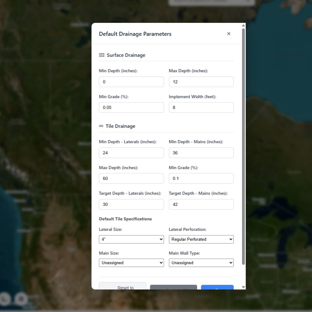
Drainage Defaults popup for configuring system-wide default parameters for all new drainage lines
Two Separate Default Systems:
Surface Drainage Defaults:
| Parameter | System Default | Applied To |
|---|---|---|
| Min Depth | 0 inches | Surface Main, Surface Tributary |
| Max Depth | 12 inches | Surface Main, Surface Tributary |
| Min Grade | 0.05% | Surface Main, Surface Tributary |
| Implement Width | 8 feet | Surface Main, Surface Tributary |
| Side Slope (H:1) | Vertical (0) | Surface Main, Surface Tributary |
The Side Slope setting affects earthwork volume calculations. Options: Vertical (no slope), 1:1 (45°), 2:1, or 3:1. Sloped sides create trapezoidal cross-sections, resulting in larger volume estimates than vertical sides.
Tile Drainage Defaults:
| Parameter | System Default | Applied To |
|---|---|---|
| Lateral Spacing | 50 feet | Report area calculations, Auto-Sizer, Offset tool |
| Min Depth - Laterals | 24 inches (2') | Tile Lateral, Tile Sub-Main |
| Min Depth - Mains | 36 inches (3') | Tile Main |
| Max Depth | 60 inches (5') | All tile types |
| Min Grade | 0.1% | All tile types |
| Target Depth - Laterals | 30 inches (2.5') | Tile Lateral, Tile Sub-Main |
| Target Depth - Mains | 42 inches (3.5') | Tile Main |
Tile Overburden Settings:
When tile depth exceeds the maximum plow depth, overburden must be excavated before the tile plow can operate. These settings control overburden volume calculations:
| Parameter | System Default | Description |
|---|---|---|
| Overburden Width | 4 feet | Bottom width of excavation trench |
| Overburden Side Slope (H:1) | Vertical (0) | Excavation side slope (Vertical, 1:1, 2:1, 3:1) |
Tile Specifications Defaults:
The Drainage Defaults popup also includes default tile specifications (used for material lists and reports):
- Lateral Size: Default 4" (options: 3", 4", 6", 8", 10")
- Lateral Perforation: Default "Regular Perforated" (options: Regular, Narrow Slot, Sock Filter)
- Main Size: Default "Unassigned" (options: Unassigned, 4"-48")
- Main Wall Type: Default "Unassigned" (options: Unassigned, Single-Wall, Dual-Wall)
Changing Defaults:
- Click Drainage Defaults button
- Modify any values in the popup (separate sections for Surface and Tile)
- Click "Save Changes" - your custom defaults are saved to browser localStorage
- All FUTURE new lines will use your custom defaults automatically
- Optional: Click "Apply to All Existing Lines" to retroactively apply new defaults to already-drawn lines
Resetting to System Defaults:
Click "Reset to System Defaults" in the Drainage Defaults popup to restore the original factory values shown in the tables above. This clears your custom defaults from localStorage.
Per-Line Parameter Overrides
While new lines automatically receive default parameters, you can override them on a per-line basis for specific drainage lines that need different settings.
Editing Individual Line Parameters:
- Select Line: Choose the drainage line from the Profile dropdown (Design tab)
- Edit Values: Manually change any of the four parameter values in the input fields
- Apply: Click "Apply & Refresh Design" button
- Saves new parameter values to that line's data
- Recalculates Best Fit grade if Best Fit was previously run
- Updates depth constraint bands on profile chart
- Mains that outlet to surface water (may need shallower max depth)
- Lines crossing roads (need deeper min depth for traffic protection)
- Steep terrain sections (can use higher min grade)
- Very flat areas (may require relaxed 0.05% min grade)
Parameters Persist Per-Line:
Once you apply custom parameters to a line:
- Values are stored in that line's data (lineData object)
- Switching to another line shows THAT line's parameters (not yours)
- Switching back shows your custom values again
- Parameters are saved in project backup files
- Parameters are included in KML exports and PDF reports
Design Parameters FAQ
Do I have to configure defaults before drawing lines?
No. The system ships with reasonable defaults for both surface and tile drainage. Most users never change them. You can start drawing immediately and adjust defaults later if needed.
What happens if I change defaults after drawing lines?
Already-drawn lines keep their existing parameters. New defaults only apply to FUTURE new lines. Use "Apply to All Existing Lines" if you want to retroactively update everything.
Why are tile mains and laterals different?
Tile mains should be installed deeper than laterals so that laterals can connect to the upper portion of the main pipe. This connection point at the top of the main provides better drainage performance and allows laterals to drain more effectively.
Can I see which lines have custom parameters vs. defaults?
No. There's no visual indicator showing whether a line uses default or custom parameters. You have to select the line and look at the parameter values.
Are defaults shared across projects?
Web version: Yes. Defaults are stored in browser localStorage, so they apply to all projects in that browser. PC version: Defaults are saved per-project and restore automatically when you reopen a project. Line-specific parameter overrides are always saved with each project on both platforms.
What if I don't click "Apply & Refresh Design" after editing parameters?
Parameter changes are NOT saved until you click the Apply button. If you edit values then switch to a different line without clicking Apply, your edits are lost.
Grade Analysis & Best Fit
Automatic grade optimization with terrain-aware depth calculations
What is Auto Best Fit?
Auto Best Fit automatically calculates the optimal drainage grade by analyzing terrain elevation and attempting to satisfy all your depth and grade constraints simultaneously. The algorithm is intelligent enough to handle both surface and tile drainage systems with different calculation strategies.
Surface vs. Tile Drainage Algorithms:
Surface Drainage (Open Ditch):
- Direction: Calculates forward from inlet (high point) to outlet (low point)
- Starting Depth: Uses Offset Depth parameter (typically 0" for surface drains)
- Strategy: Maintains minimum grade, follows terrain when natural slope exceeds minimum
- Typical Use: Open ditches, grassed waterways, surface channels
Tile Drainage (Subsurface):
- Direction: Calculates forward from inlet (high point) to outlet (low point)
- Starting Depth: Uses Offset Depth parameter as Target Depth (e.g., 30" for laterals, 42" for mains)
- Strategy: Starts at inlet at Target Depth, maintains minimum grade, tries to avoid depth violations
- Optimization: If violations occur, automatically tests adjusted inlet depths to find violation-free solution
- Output: Calculates Required Starting Depth at outlet for construction planning
How Auto Best Fit Works
Auto Best Fit automatically calculates the optimal grade for your drainage line by analyzing terrain elevation and attempting to satisfy all your depth and grade constraints. Best Fit runs automatically when you finish drawing a new line, and you can also manually trigger it using the "Auto Best Fit" button.
Automatic Calculation on New Profiles:
When you finish drawing a new drainage line (double-click to complete), Auto Best Fit runs automatically:
- System applies default parameters based on drainage type (Surface/Tile, Main/Lateral/etc.)
- Auto Best Fit immediately calculates optimal grade using those parameters
- Profile chart displays with the calculated grade line already drawn
- You see the result immediately - no manual steps required
Manually Running Best Fit:
You can also manually run (or re-run) Best Fit on an existing line by clicking the "Auto Best Fit" button in the Grade Analysis toolbar:
- Select a drainage line from the Profile dropdown
- Click the "Auto Best Fit" button
- System immediately runs the calculation using outlet (start) and inlet (end) points
- Any existing grade line is cleared and replaced with the new Best Fit result
- Profile chart updates with the new grade line and statistics
This is useful when you've drawn a Guided or Freeform grade but want to see what the automatic optimization would produce, or when you want to recalculate after making parameter changes.
What Auto Best Fit Displays:
After calculation completes, the profile chart shows:
- Red grade line: The calculated drain invert elevation along the profile
- Green/Magenta bands: Min Depth (green) and Max Depth (magenta) constraint zones
- Red X markers: Depth violation points where calculated depth exceeds min/max constraints
- Profile statistics: Grade percentage, depths (min/avg/max), total fall, line length
- Required Starting Depth: (Tile drainage only) The depth at the outlet needed to maintain design throughout

Profile chart displaying Best Fit grade line (red), terrain elevation (blue), depth constraint zones (green/magenta), and design statistics
Re-running Best Fit After Parameter Changes:
If the initial result has depth violations or connection violations, adjust your parameters and re-run:
- Edit Parameters: Adjust Min Grade, Target Depth, Min Depth, or Max Depth values in the Design Parameters card
- Click "Apply & Refresh Design": This button saves the new parameters AND automatically re-runs Auto Best Fit
- Review Updated Result: Check if violations are resolved on the refreshed profile chart
- Repeat if Needed: Continue adjusting parameters and clicking Apply until design is acceptable
Target Depth is just a preference - the algorithm automatically searches for workable solutions within your Min/Max Depth range. If violations occur, the constraints are too narrow for the terrain.
- Too Shallow (above green line): DECREASE Min Depth to allow shallower installation, or DECREASE Min Grade % to allow flatter grades
- Too Deep (below magenta line): INCREASE Max Depth to allow deeper installation, or DECREASE Min Grade % to prevent line from diving too deep
- Connection Violations (laterals): Adjust Target Depth to change the outlet elevation where the lateral connects to the main
Apply & Refresh Design Button
The "Apply & Refresh Design" button (blue primary button with sync icon) is the most important control for updating your design after making parameter changes.
What It Does:
Clicking "Apply & Refresh Design" performs the following operations in sequence:
- Saves Parameters: Stores all four parameter values (Min Grade, Offset Depth, Min Depth, Max Depth) to the selected line's data
- Recalculates Best Fit: If you previously ran Best Fit on this line, it automatically re-runs the Best Fit algorithm with your new parameters, recalculating the entire grade line and Required Starting Depth
- Updates Depth Constraints: Redraws the Min Depth (green) and Max Depth (magenta) constraint lines on the profile chart
- Recalculates Violations: Checks the new grade line against new Min/Max Depth values and updates red X violation markers
- Updates Connection Validation: Recalculates connection status for all lines (checks if lateral outlets are above/below main elevations)
- Updates Status Colors: Refreshes dropdown colors and map icons based on new validation results
When to Use It:
You MUST click "Apply & Refresh Design" after:
- Changing Min Grade % value
- Changing Offset Depth (Target Depth) value
- Changing Min Depth constraint
- Changing Max Depth constraint
- Adjusting any parameter for a line that already has a Best Fit grade
Example Workflow:
Suppose you ran Best Fit on a tile lateral and got depth violations (red X markers). To fix:
- Increase Max Depth from 48" to 60" in the Design Parameters
- Click "Apply & Refresh Design"
- System automatically re-runs Best Fit with new 60" max depth
- Violations disappear if the line now stays within 60" max
- Status color updates to green ✓ (all checks pass)
Guided Grade Mode
Guided mode lets you manually draw a grade line by clicking points on the profile chart, while the system enforces your minimum grade constraint between vertices and automatically extends the line to the outlet. This is ideal when you need manual control but still want grade rules respected.
How to Draw Guided Grades:
- Select a drainage line from the Profile dropdown
- Click the "Guided" button in the Grade Analysis toolbar
- Button changes to "Finish Drawing" (orange) to indicate drawing mode is active
- Click on the profile chart to place grade line vertices:
- Vertices snap to the nearest terrain data point (elevation sample)
- Minimum grade is enforced between each vertex - the line will not go flatter than your Min Grade setting
- The grade line automatically extends from your last vertex to the outlet at minimum grade
- Click near the far end to snap to the inlet
- Place as many vertices as needed for your design
- Click "Finish Drawing" when complete
- System automatically runs validation checks:
- Connection validation (if lateral/secondary drain)
- Depth violation detection (red X markers if outside Min/Max Depth)
After Drawing:
Once a Guided grade is drawn, changing design parameters (Min Grade, Min/Max Depth) and clicking "Apply & Refresh Design" will redraw the grade line with the new constraints, recalculating depth violations and statistics in real time.
Freeform Grade Mode
Freeform mode gives you complete creative control over grade line design. Click anywhere on the profile chart to place vertices at exact coordinates, then drag them freely to shape your grade line. There is no snapping to terrain points, no minimum grade enforcement, and no auto-extension - you have full control.
How to Draw Freeform Grades:
- Select a drainage line from the Profile dropdown
- Click the "Freeform" button in the Grade Analysis toolbar
- Button changes to "Finish Freeform" (orange) to indicate freeform mode is active
- Click anywhere on the profile chart to place vertices:
- Vertices are placed at the exact X/Y coordinate you click - no snapping
- Straight line segments connect your vertices in order
- You must place at least two vertices (start and end of the grade line)
- Drag vertices to adjust position after placement:
- Click and hold on any existing vertex to drag it
- The grade line updates in real time as you drag
- Depth violations update in real time on both the chart (red X markers) and the map
- Click "Finish Freeform" when complete
Real-Time Violation Feedback:
As you drag vertices, the system continuously checks for depth violations and displays red X markers on both the profile chart and the map. This lets you see exactly where your grade line goes too shallow or too deep, and adjust in real time to find the optimal design.
Profile Chart Elements
The elevation profile chart displays multiple data series with specific colors and display order:
Chart Layers (Bottom to Top):
- Blue line (Elevation Profile): Natural terrain elevation sampled along the drainage path
- Green line (Min Depth Line): Shows the shallowest allowable drain elevation (terrain minus Min Depth)
- Magenta line (Max Depth Line): Shows the deepest allowable drain elevation (terrain minus Max Depth)
- Orange shaded areas (Overburden): Regions where tile depth exceeds Max Depth, indicating pre-excavation needed
- Red line (Grade Line or Best Fit Line): Your designed drainage line elevation
- Red X markers (Depth Violations): Points where the grade line violates Min or Max Depth constraints
- Green/Yellow connection dots (if connections exist): Shows where secondary drains connect to this main
- Dashed vertical lines (Pipe Size Segments): When stepped sizing is applied, dashed lines mark where pipe size changes with size labels
- Station labels: At grade change points, station values (e.g., 2+50) appear for construction reference
- Freeform vertices (blue circles): In Freeform grade mode, draggable vertex handles appear at each grade point
Interactive Features:
- Hover for Details: Hover your mouse over any point on the chart to see precise values at that location
- Zoom: Click and drag a selection box to zoom in on a region
- Resize: Drag the handle at the bottom edge of the chart to make it taller or shorter
FAQ
Why does my tile lateral show a Required Starting Depth?
Required Starting Depth (shown after running Best Fit on tile drainage) tells you how deep the outlet end needs to be to achieve the calculated grade. For laterals connecting to mains, this helps you determine if the lateral will properly connect above the main pipe as required.
What if Best Fit shows violations no matter what I try?
Some terrain is simply too steep or irregular to satisfy all constraints. Options: (1) Widen your Min/Max Depth range, (2) Split the line into two shorter segments with a junction, (3) Accept violations and plan for custom construction adjustments, (4) Reroute the line to avoid problem areas.
Can I edit the red grade line directly on the chart?
Yes, in Freeform mode! Click "Freeform" to enter freeform grade drawing, then drag vertices to reshape the grade line interactively. In Guided and Best Fit modes, the grade line is calculated from parameters - adjust your Design Parameters and click "Apply & Refresh Design" to recalculate.
Do parameter changes automatically update the grade line?
No. You must explicitly click "Apply & Refresh Design" to trigger recalculation. This prevents accidental changes and gives you control over when to recompute.
Design Statistics
Real-time performance metrics for your drainage designs
What are Design Statistics?
Design Statistics provide comprehensive quantitative analysis of your drainage line designs. After drawing a line and applying a grade (Best Fit, Guided, or Freeform), the statistics panel displays critical metrics including depths, grades, lengths, and volumes. These metrics help you validate your design meets project requirements and assist with construction planning and cost estimation.
Statistics vary by drainage type and position in the system:
- Surface Mains show outlet depth and volume metrics
- Surface Tributaries show connection depth instead of outlet depth
- Tile Mains show starting depth and required starting depth
- Tile Laterals/Submains show connecting depth and required starting depth
Understanding Depth Metrics
Depth metrics are the most critical statistics for drainage design. Different depth values appear depending on whether you're designing a surface or tile drain, and whether it's a main line or a secondary line connected to a main.
Outlet Depth
When it appears: Surface mains (non-connected lines)
What it is: The depth of THIS drainage line at the outlet point (where water exits the system). This is the depth at the starting point of the line where it discharges.
How it's calculated: Ground elevation minus grade line elevation at the first point of this line, converted to inches.
Why it matters: Tells you how deep to excavate at the discharge point. This is the actual depth needed for construction at the outlet.
S1 shows "Outlet Depth: 4.00 in" - excavate 4 inches at the outlet point.
Connection Depth
When it appears: Surface tributaries (connected to a surface main)
What it is: The depth of the MAIN line's grade at the point where this tributary connects to it. This is NOT the tributary's own depth - it's showing how deep the main is at the connection location.
How it's calculated: System finds the main line, locates the connection point on it, then calculates: main's ground elevation minus main's grade line elevation at that point, converted to inches.
Why it matters: Shows how deep the main is where your tributary ties in. Your tributary must reach at least this depth to connect properly.
S1-TR1 shows "Connection Depth: 4.00 in" - the main S1 is 4 inches deep at the connection point.
Starting Depth
When it appears: Tile mains (non-connected lines)
What it is: The actual depth of THIS tile main at its starting point, based on the terrain elevation and the calculated grade line.
How it's calculated: Ground elevation minus grade line elevation at the first point of this line, converted to inches.
Why it matters: Compare this to Required Starting Depth (shown above it). If they match closely, your design is feasible. If they differ significantly, you may need to adjust Target Depth, widen Min/Max Depth range, or reroute.
T1 shows:Required Starting Depth: 42.00 in (what you need from design)
Starting Depth: 42.00 in (what terrain provides)
These match perfectly - design is feasible.
Connecting Depth
When it appears: Tile laterals and submains (connected to a tile main)
What it is: The depth of the MAIN line's grade at the point where this lateral/submain connects to it. This is NOT the lateral's own depth - it's showing how deep the main is at the connection location.
How it's calculated: System finds the main line, locates the connection point on it, then calculates: main's ground elevation minus main's grade line elevation at that point, converted to inches.
Why it matters: Shows how deep the main is where your lateral ties in. The lateral's outlet must reach the connection point. Note this is often deeper than the lateral's Target Depth because the main is already deep at that location.
T1-L1 shows:Required Starting Depth: 30.00 in (lateral outlet depth needed)
Connecting Depth: 42.00 in (how deep main is)
Target Depth: 30.00 in (your design goal)
The lateral's outlet is at 30" while the main is 42" deep at that point - the lateral connects to the upper portion of the main, which is ideal for drainage flow.
Required Starting Depth
When it appears: All tile drains (mains, submains, laterals) after running Best Fit
What it is: The depth required at the starting point based on backward calculation from the connection/outlet point. This represents the optimal starting depth needed to achieve your target grade and reach the connection depth.
How it's calculated: Backward best-fit algorithm: starts from the connection point (or outlet), works backward along the line applying the minimum grade, calculates what depth is needed at the start to maintain grade while respecting Min/Max depth constraints.
Why it matters: This is the DESIGN REQUIREMENT - what depth you NEED at the start to achieve proper grade. Always displayed in bold as the primary metric. Compare it to Starting Depth (mains) or Connecting Depth (laterals) to verify feasibility.
Target Depth
When it appears: All tile drains (mains, submains, laterals)
What it is: Your design target depth - this is the Offset parameter you specified in Design Parameters.
How it's calculated: Directly from the Offset field in Design Parameters.
Why it matters: This is your desired burial depth for the tile drain. Best Fit tries to maintain this depth while respecting Min/Max constraints and minimum grade requirements. If violations occur, you may need to adjust this target or widen your Min/Max range.
Understanding Performance Metrics
Average Depth
What it is: The distance-weighted average depth of the drainage line along its entire length.
How it's calculated: For each segment between elevation points, calculate the average cut depth, multiply by segment length, sum all segments, divide by total length.
Why it matters: Provides a single representative depth value for the entire line. Useful for quick cost estimation and comparing alternative routes.
Min Depth / Max Depth
What they are: The shallowest and deepest points along the entire drainage line.
How they're calculated: System tracks depth at every elevation point (ground minus grade), records minimum and maximum values encountered.
Why they matter: Show the range of excavation depths required. Large ranges may indicate challenging terrain. Compare these to your Min/Max Depth constraints to verify compliance.
Average Grade
What it is: The overall slope of the drainage line expressed as a percentage.
How it's calculated: (Total elevation change ÷ Total horizontal distance) × 100
Why it matters: Validates your design meets minimum grade requirements. Too low and drainage may be sluggish; too high and erosion may occur. Typical agricultural surface drains: 0.2-0.5%. Pattern tile: 0.1-0.2%.
Run Length
What it is: The total horizontal distance of the drainage line.
How it's calculated: Directly from the line's measured length in feet (from linesData).
Why it matters: Essential for material quantity calculations, cost estimation, and verifying the line length meets project requirements.
Total Volume (Surface Drains Only)
What it is: The total volume of material to be excavated, expressed in cubic yards.
How it's calculated: Uses trapezoidal cross-section based on your Side Slope setting:
- Vertical (0): Rectangle - bottom width × depth × length
- With side slope: Trapezoid - ((bottom + top width) / 2) × depth × length, where top width = bottom + (2 × depth × slope ratio)
Why it matters: Critical for earthwork cost estimation. Side slopes significantly increase volume - a 2:1 slope can nearly double the volume compared to vertical sides.
• Vertical: 100 × 2 × 8 ÷ 27 = 59.3 yd³
• 2:1 slope: top = 8 + (2 × 2 × 2) = 16 ft, area = 12 × 2 = 24 ft², volume = 100 × 24 ÷ 27 = 88.9 yd³
Overburden Stats (Tile Drains Only)
What it is: When tile depth exceeds Max Depth (typical plow limit), the system calculates overburden - material that must be pre-excavated so the tile plow can operate at normal depth.
Stats displayed (in orange):
- Overburden Length: Total linear feet where depth exceeds Max Depth
- Overburden Volume: Cubic yards of material to excavate, using your configured width and side slope
Why it matters: Overburden excavation is typically done by backhoe before the tile plow arrives. This separate earthwork has different costs and scheduling requirements than standard tile installation.
Statistics by Drainage Type
The specific statistics displayed vary based on drainage type (surface vs. tile) and position (main vs. secondary). Here are the four main configurations:
Surface Main Line
Note: Shows Outlet Depth (depth at discharge point) and includes Total Volume calculation for earthwork estimation.
Surface Tributary/Secondary
Note: Shows Connection Depth (main line's depth at connection point) instead of Outlet Depth. This is the depth the tributary must reach to connect properly.
Tile Main Line
Note: Shows Required Starting Depth and Starting Depth for design validation. When Max Depth (68.20 in) exceeds the 60" plow limit, overburden stats appear in orange showing pre-excavation requirements.
Tile Lateral/Submain (Connected to Main)
Note: Shows Required Starting Depth and Connecting Depth (main line's depth at connection). Connecting Depth indicates how deep the main is where this lateral ties in.
Using Statistics for Design Validation
Design Statistics help you validate and optimize your drainage designs. Here's how to interpret and act on the metrics:
Check Depth Feasibility
For tile drains: Compare Required Starting Depth to Starting Depth (mains) or Connecting Depth (laterals). Large discrepancies indicate the design may not be achievable with current parameters. Adjust Target Depth, widen Min/Max Depth range, or reroute the line.
Verify Grade Requirements
Surface drains: Average Grade should typically be 0.2-0.5%. Below 0.2% risks poor drainage; above 0.5% may cause erosion.
Tile drains: Average Grade should typically be 0.1-0.2%. Pattern tile can go as low as 0.05% in very flat terrain.
If Average Grade is too low, increase grade in Design Parameters or reroute to steeper terrain. If too high, consider reducing grade or using erosion control measures.
Estimate Costs
Surface drains: Total Volume directly translates to earthwork costs. Multiply by your local excavation rate ($/yd³).
Tile drains: Use Run Length and tile specifications to calculate material costs. The system can auto-calculate this in the PDF Report Generator.
Compare Alternatives
When evaluating multiple design options, statistics help you compare:
- Excavation depth: Lower Average Depth = lower construction cost
- Length: Shorter Run Length = less material and labor
- Volume: Lower Total Volume = lower earthwork cost
- Grade: Grade closer to target = better long-term performance
Common Questions
Why don't statistics appear immediately after drawing a line?
Statistics require a grade line. After drawing a line, click "Best Fit", "Guided", or "Freeform" to create a grade, then statistics will populate. Without a grade line, there's no depth or volume data to calculate.
What if Required Starting Depth and Starting Depth don't match?
This is common and indicates a design challenge. Required Starting Depth shows what you NEED; Starting Depth shows what you HAVE. To resolve: (1) Increase Target Depth, (2) Widen Min/Max Depth range, (3) Reduce minimum grade requirement, or (4) Reroute to different terrain.
Why is Connecting Depth sometimes deeper than my target?
Connecting Depth reflects the main line's depth at the connection point - which you don't control from the secondary line. If the main is deeper than expected, your secondary line must reach that depth to connect. Consider this when setting Target Depth for secondaries.
Do statistics account for tile size or trench width?
For tile drains: No, statistics show cut depth only. Actual trench excavation will be deeper (add tile diameter + bedding). For surface drains: Volume calculations use the configured trench top width from drainage defaults.
Can I export statistics for reporting?
Yes. Use the PDF Report Generator in the Import/Export tab. It includes all design statistics plus materials, flow rates, and cost estimates in a professional format suitable for clients or contractors.
Depth Violation Detection
Automatic identification of depth constraint violations
What are Depth Violations?
Depth violations occur when your designed drainage line (Best Fit, Guided, or Freeform grade) goes deeper or shallower than the Min/Max Depth constraints you specified in Design Parameters. The system automatically detects these violations and displays warning markers so you can address them before construction.
Two Types of Violations:
- Too Shallow: Drain depth at some point is less than Min Depth (e.g., drain is 18" deep but Min Depth is 24")
- Too Deep: Drain depth at some point is greater than Max Depth (e.g., drain is 66" deep but Max Depth is 60")
Both violation types are treated equally serious - they indicate the design doesn't meet your constraints and may require parameter adjustment or terrain modification.
Visual Indicators
Depth violations are shown with prominent red markers in three locations:
1. Profile Chart Markers (Red X)
Appearance: Red crossRot markers (X shapes, rotated 45°) appear directly on the profile chart at the exact distance where violations occur.
Location: Overlaid on the Best Fit red line at violation points, displayed on top of all other chart elements so they're always visible.
Tooltip: Hover over any red X to see details: depth value at that point, violation type (too shallow/too deep), and the Min/Max Depth constraint that was violated.
2. Map Markers (Red X)
Appearance: Red X markers appear at the geographic location of each violation point along the drainage line on the map.
Persistence: Map violation markers are persistent - they stay visible even when you switch to viewing a different line's profile. This lets you see ALL violations across your entire drainage system at once.
Purpose: Helps you quickly identify which physical areas of your field have depth issues, especially useful when you have multiple lines with violations.
3. Profile Dropdown Colors (Orange Text)
Appearance: Lines with depth violations (but no connection issues) appear in orange text in the Profile dropdown.
Combined Issues: If a line has BOTH depth violations and connection issues, it appears in red text instead.
See the "Connection Validation" section for full details on dropdown color codes.

Surface ditch example showing depth violations (red X markers) where the design exceeds maximum allowable depth - would require increasing max depth constraint or finding an alternative route
When Violations are Calculated
The system automatically checks for depth violations at these times:
1. After Running Best Fit
As soon as you click the second point to run Best Fit, the algorithm:
- Calculates the grade line and depth at every point
- Compares each depth value against Min/Max Depth constraints
- Creates violation markers for any points outside the allowed range
- Displays red X markers on chart and map
- Updates the dropdown status color to orange (depth issues only) or red (depth + connection issues)
2. After Clicking "Apply & Refresh Design"
When you change parameters and click "Apply & Refresh Design":
- If Best Fit was previously run, it re-runs with new parameters
- Recalculates violations with new Min/Max Depth values
- Updates/removes violation markers as appropriate
- Updates status colors in dropdown and map icons
For example: If you had violations at Max Depth = 48", then increase it to 60" and click Apply & Refresh, violations may disappear if the line now fits within the new constraints.
3. After Restoring a Project
When you load a saved project file, violations are restored from the saved lineData so you immediately see which lines had depth issues when the project was saved.
Fixing Depth Violations
Here are the most effective strategies for resolving depth violations, in order from simplest to most complex:
Strategy 1: Widen Depth Constraints (Simplest)
- Increase Max Depth (if violations are "too deep") OR decrease Min Depth (if violations are "too shallow")
- Click "Apply & Refresh Design"
- Best Fit automatically recalculates and violations may disappear
When to use: First option to try. Often the quickest fix if your constraints were too strict.
Strategy 2: Adjust Target Depth / Offset
- Change the Offset Depth (Target Depth) parameter - make it deeper or shallower to shift the entire profile
- Click "Apply & Refresh Design"
- Best Fit recalculates starting at the new target depth
When to use: If the entire line is consistently too deep or too shallow, shifting the target depth can solve it.
Strategy 3: Change Minimum Grade
- Decrease Min Grade % if violations are "too deep" (allows flatter grades that don't drop as much)
- Increase Min Grade % if violations are "too shallow" (forces steeper grades that drop more)
- Click "Apply & Refresh Design"
When to use: If terrain dictates the grade and you have flexibility in minimum grade requirements.
Strategy 4: Split the Line
If a long line has violations in one section but not others:
- Delete the problematic line
- Draw two shorter lines instead, splitting at the problem area
- Run Best Fit on each segment independently
- Each segment can now use different parameters or grades
When to use: Terrain break or major grade change makes one continuous line impossible to design within constraints.
Strategy 5: Reroute the Line
If violations persist no matter what:
- Delete the line
- Draw a new line along a different path that avoids steep areas or problem terrain
- Run Best Fit on the new route
When to use: The terrain is simply unsuitable for drainage along that path. A different route may have better topography.
Strategy 6: Accept Violations (Last Resort)
Sometimes violations are unavoidable:
- Plan for custom construction adjustments (deeper trench, fill low areas, etc.)
- Note the violation locations on your construction plans
- Coordinate with equipment operators to handle problem areas
When to use: All other strategies exhausted, and construction flexibility exists.
FAQ
Do depth violations prevent me from exporting my design?
No. Depth violations are warnings, not hard errors. You can export designs, generate reports, and save projects even with violations present. They're meant to alert you to review those areas, not block your work.
Why do violations appear on the map but not in the chart?
Chart violations only show for the currently selected line (the one whose profile you're viewing). Map violations show for ALL lines simultaneously so you can see the full system. If you see map violations but no chart violations, you're probably viewing a different line's profile - switch to the line with violations to see its chart markers.
Can I manually delete individual violation markers?
No. Violation markers are automatically managed by the system. To remove them, you must fix the underlying issue (adjust parameters, reroute line, etc.) and click "Apply & Refresh Design".
What if I get "too deep" violations near the outlet of a tile lateral?
This is common on steep terrain. The lateral needs to maintain minimum grade and ends up going deeper than Max Depth at the outlet. Options: (1) Increase Max Depth, (2) Shorten the lateral, (3) Increase Min Grade to steepen the line (causes it to drop faster and reach the main sooner, reducing outlet depth), (4) Move the inlet location uphill less.
Do violations affect flow calculations or tile sizing?
No. Flow calculations and tile sizing are based on the designed grade line regardless of whether violations exist. Violations are a construction/feasibility concern, not a hydraulic concern.
Connection Validation
Post-design verification of lateral-to-main connections
Connection Enforcement vs. Connection Validation
It's critical to understand the difference between these two systems - they work at different stages of the design process:
Connection Enforcement (During Drawing):
- When: Active while you're drawing secondary drains (laterals, tributaries, sub-mains)
- What it does: Forces you to click within 30 feet of a compatible main drain, prevents drawing connections that are too far away
- Purpose: Ensures geographic proximity - makes sure lines physically connect
- Validation: Based on map distance only, no elevation checking
Connection Validation (After Best Fit):
- When: Active after you run Best Fit, Guided, or Freeform grade and click "Apply & Refresh Design"
- What it does: Checks the ELEVATION difference between the lateral outlet and the main at the connection point
- Purpose: Ensures hydraulic validity - laterals must connect to the upper portion of the main pipe, not below it
- Validation: Based on designed elevations (Best Fit lines), not terrain
How Connection Validation Works
After you run Best Fit (or create a Guided/Freeform grade) on both a main line and its connected secondary drains, the system performs elevation-based validation:
The Validation Rule:
For tile drainage, laterals should connect to the upper portion of the main pipe for optimal drainage performance. The validation check compares designed elevations at the connection point:
- Main Elevation: System calculates the main drain's designed elevation (from its Best Fit line) at the distance where the lateral connects
- Lateral Elevation: System gets the lateral's designed elevation at its outlet point (index 0, the connection end)
- Elevation Difference: Calculates:
Lateral Elevation - Main Elevation - Pass/Fail Decision:
- PASS (Green ✓): If lateral is within 1 inch or SHALLOWER than main (
diff >= -0.0833 feet) - FAIL (Red ✗ or Purple ✗): If lateral is more than 1 inch DEEPER than main (
diff < -0.0833 feet)
- PASS (Green ✓): If lateral is within 1 inch or SHALLOWER than main (
When Validation Runs:
Connection validation is automatically triggered:
- After running Best Fit on any line
- After clicking "Apply & Refresh Design" on any line
- After restoring a project file
- After deleting or modifying any line
The system checks ALL connections in the entire drainage network every time, not just the current line. This ensures the status colors and icons are always current.
Visual Indicators
Connection validation status is displayed in two locations with a comprehensive color-coded system:
1. Profile Dropdown Colors
The Profile dropdown (Design tab) shows each drainage line with color-coded text indicating its validation status. This is the primary way to quickly assess your entire drainage system's health:
| Color | Meaning | Issues |
|---|---|---|
| Green | All checks pass | No depth violations, no connection issues. Ready for construction. |
| Orange | Depth violations only | Has depth violations (too deep or too shallow), but all connections are valid. |
| Purple | Connection issues only | One or more laterals connect too deep below the main, but no depth violations on the line itself. |
| Red | Both issues | BOTH depth violations AND connection issues. Most critical status. |
| Black | No grade line set | Line has been drawn but Best Fit not run yet. No validation possible without a design. |
2. Map Validation Icons
Each drainage line's label on the map shows a validation icon next to its hierarchical ID (e.g., "T1-L1 ✓"). The icon indicates the line's validation status:
| Icon | Color | Meaning |
|---|---|---|
| ✓ | Green | All checks pass (matches green dropdown status) |
| ⚠ | Orange | Depth violations only (matches orange dropdown status) |
| ✗ | Purple | Connection issues only (matches purple dropdown status) |
| ✗✗ | Red | Both depth violations AND connection issues (matches red dropdown status) |
| (none) | - | No grade line set yet - no validation possible |
Map icons appear next to the hierarchical ID label at the midpoint of each drainage line. They update automatically whenever validation status changes.
Fixing Connection Issues
If you see purple (connection issues only) or red (connection + depth issues) status, here are strategies to resolve connection problems:
Strategy 1: Adjust Main Line Depth (Simplest)
If the main line is too deep at the connection point, make it shallower:
- Select the main line from the Profile dropdown
- Decrease the main's Target Depth (Offset Depth) by 6-12 inches
- Click "Apply & Refresh Design" to recalculate the main's Best Fit
- Check if the status changes from purple/red to green/orange
Why this works: Raising the main line elevation at all points brings it closer to or above the lateral outlet elevation.
Strategy 2: Adjust Lateral Depth
If the lateral is too deep at its outlet, make it shallower:
- Select the lateral from the Profile dropdown
- Decrease the lateral's Min Depth (allows shallower installation)
- Click "Apply & Refresh Design" to recalculate
- Check if the lateral's outlet elevation rises enough to connect properly
Limitation: Laterals often need to be at least 24" deep minimum for tile drainage standards, so you may not have much adjustment room here.
Strategy 3: Increase Lateral Grade
Steeper lateral grade causes it to drop faster from inlet to outlet, which can paradoxically help:
- Select the lateral from the Profile dropdown
- Increase the lateral's Min Grade % (e.g., from 0.1% to 0.2%)
- Click "Apply & Refresh Design"
- The lateral drops faster, reaching the main sooner at a shallower depth
When to use: If the lateral is long and terrain allows steeper grades.
Strategy 4: Shorten the Lateral
If a lateral is too long, it accumulates too much drop and ends up too deep:
- Delete the lateral
- Redraw it with the inlet closer to the main (shorter length)
- Run Best Fit on the new shorter lateral
- Check if it now connects at an acceptable elevation
Trade-off: Shorter laterals drain less area. You may need to add more laterals to cover the same field area.
Strategy 5: Move Connection Point on Main
Sometimes moving where the lateral connects to the main can find a shallower spot:
- Delete the lateral
- Redraw it connecting to a different point along the main (farther upstream where the main may be shallower)
- Run Best Fit on the repositioned lateral
When to use: If the main has varying depth along its length and some connection points are more favorable than others.
Strategy 6: Accept Connection Issue (Rare)
In some cases, you may need to accept a connection issue and plan for custom construction:
- Install the lateral slightly shallower than designed at the outlet
- Use a riser or junction box to accommodate the elevation difference
- Modify the main installation depth locally to be deeper at that connection
When to use: All design adjustments exhausted, construction flexibility exists, or terrain makes a proper connection impossible without major rerouting.
Connection Depth Calculation
For secondary drains (laterals, tributaries, sub-mains) that connect to main lines, the system stores a special "Connection Depth" value after validation runs. This represents the depth of the main pipe at the connection point and is used for:
- Reports: PDF reports show connection depth for each lateral to help construction crews know how deep to install junctions
- Validation: Used internally to calculate whether the lateral outlet is above or below the main at the connection
- Planning: Helps you assess if junctions are practical (e.g., a 72" deep connection may not be feasible)
How Connection Depth is Calculated:
- System finds the main line's terrain elevation at the connection point (interpolated from elevation data)
- System finds the main line's designed elevation at the connection point (interpolated from Best Fit line)
- Connection Depth = Terrain Elevation - Designed Elevation
- Value is stored in inches and shown in reports
Connection Depth is distinct from the lateral's Required Starting Depth (which is the depth at the lateral's outlet, not the main's depth).
FAQ
Why does my lateral show purple (connection issue) even though it's within 30 feet of the main?
Connection Enforcement (30-foot rule) and Connection Validation (elevation check) are separate. You passed enforcement when you drew the line, but after running Best Fit, the designed elevations put the lateral too deep relative to the main. This is an elevation problem, not a distance problem.
Can a line have orange status (depth violations) but still be usable?
Yes. Orange means depth violations but valid connections. The line may work hydraulically (connections are good) but have construction challenges (too deep or too shallow). Purple/red status indicates hydraulic problems (bad connections) which are more critical.
What if the main line shows purple/red status?
This means one or more of its connected laterals are too deep at their connection points. The main itself may be fine, but it's flagged to alert you that its laterals have connection issues. Select each lateral individually to see which ones are problematic.
Why do status colors sometimes change when I edit a different line?
Connection validation checks the entire drainage network, not just the current line. If you adjust a main line's depth, all its connected laterals' validation status may change because the main's elevation at their connection points changed. Similarly, adjusting one lateral's depth doesn't affect others, but the main's status may update to reflect that one lateral is now valid.
Do I need to fix all lines to green before exporting?
No. You can export designs with any status. Green is the ideal goal (no issues), but orange/purple/red designs can still be exported - they just require more attention during construction. The color codes are guidance, not hard blockers.
What does "no icon" mean on a map label?
If a drainage line label shows just the hierarchical ID with no validation icon, it means Best Fit has not been run on that line yet (black status in dropdown). No design = no validation possible. Run Best Fit to get a validation icon.
Tile Sizing & Specifications
Automatically calculate main pipe sizes and manage tile specifications
Overview
The tile sizing system handles two distinct tasks:
- Auto Size Tile Mains: Wizard-based automatic sizing for tile mains and sub-mains using flow calculations
- Tile Specifications: Manual specification of laterals and unsized mains (size, wall type, perforation)
Auto Size Tile Mains (Wizard)
The Auto Size Tile Mains wizard automatically calculates pipe sizes for ALL tile mains and sub-mains in your drainage system based on contributing area, drainage coefficient, and grade.
How It Works:
- Click "Auto Size Tile Mains" button in Design tab (below profile chart)
- Enter Parameters:
- Drainage Coefficient: Select 1/8", 1/4", 3/8" (default), 1/2", 3/4", or 1" per 24 hours
- Average Drain Spacing: Distance between lateral drains in feet (pre-fills from your saved lateral spacing default, range: 10-200ft)
- Click "Start Sizing" to begin wizard
- For Each Main/Sub-Main: System shows popup with:
- Contributing area calculation (acres)
- Average grade (%)
- 2-3 sizing options (buttons)
- Select Size Option or click "Skip" to leave unassigned
- Wizard Completes: Shows summary of sized vs skipped lines

Auto Pipe Sizer wizard displaying calculated sizing options for a tile main with contributing area and grade information
Stepped Main Sizing BETA
Stepped main sizing calculates variable pipe sizes along a single main line, using larger pipe at the outlet (where all flow accumulates) and progressively smaller pipe toward the inlet (where less area drains). This can reduce material costs compared to using a single size for the entire main.
How It Works:
When enabled, the system divides the main into segments at each lateral connection point. Starting from the outlet, it calculates the cumulative contributing area at each connection and sizes the pipe for that segment based on the flow at that point.
Enabling Stepped Sizing:
- Click "Auto Size Tile Mains" to open the sizing wizard
- Check the "Enable stepped main sizing" checkbox
- Set your Drainage Coefficient and Average Drain Spacing as usual
- Click "Start Sizing"
- For each main, a Stepped Sizing Review popup appears showing:
- Each segment with station range, length, contributing area
- Calculated pipe size, wall type, and perforation for each segment
- Editable dropdowns to override size, wall type, or perforation per segment
- Review and adjust segments as needed, then click "Apply Stepped Sizing"
Segment Visualization:
After applying stepped sizing, the elevation profile chart displays:
- Dashed vertical lines at each segment boundary (where pipe size changes)
- Size labels on each segment (e.g., "12\" SW", "8\" SW")
- The visualization updates when you switch between lines
In PDF Reports:
Stepped sizing data appears in the Main Lines Analysis section as a breakdown table showing each segment's station range, length, pipe size, wall type, perforation, and area drained. The profile chart in the report also shows the segment boundaries.
Contributing Area Calculation
For each main or sub-main, the system automatically calculates contributing area from connected drainage lines:
Non-Perforated Mains:
- Collects ALL laterals and sub-mains that drain to this main
- Sums total length of all descendants in feet
- Area (acres) = (Total Length × Drain Spacing) ÷ 43,560
- Example: 10 laterals × 500ft each = 5,000ft → (5,000ft × 50ft spacing) ÷ 43,560 = 5.74 acres
Perforated Mains (if selected):
- Same as above, PLUS adds the main's own drainage contribution
- Assumes main drains half the lateral spacing on each side (e.g., 25ft each side for 50ft spacing)
- Area (acres) = (Total Lateral Length + Main Length) × Drain Spacing ÷ 43,560
Sizing Options Presented
For each main/sub-main, the wizard calculates and presents 2-3 sizing options based on wall type and perforation:
1. Single-Wall Non-Perforated (Green Button)
- Always shown
- Uses only lateral contributing area (no main drainage)
- Standard corrugated single-wall pipe
- Best for collection mains that don't directly drain soil
2. Single-Wall Perforated (Cyan Button)
- Only shown if calculated size ≤ 15 inches
- Includes main's own drainage contribution in area calculation
- After clicking, shows perforation type picker:
- Regular Perforated: Standard perforations
- Narrow Slot: Narrow slot openings (fine soils)
- Sock Filter: Fabric sock wrapped pipe
- Best when main also needs to drain soil along its length
3. Dual-Wall (Grey Button)
- Always shown
- Smooth interior wall, corrugated exterior
- Always non-perforated (dual-wall mains don't come perforated)
- Higher flow capacity due to smoother surface (lower roughness coefficient)
- Best for high-flow collection mains or challenging grades
Flow Calculation Details
The sizing algorithm uses Manning's equation with size-dependent roughness coefficients:
Flow Rate (Q):
Q (cu ft/sec) = Area (acres) × Drainage Coefficient (in/24hr) × Conversion Factor
Conversion Factor = 43,560 ÷ 12 ÷ 3,600 ÷ 24 = 0.0423
Example: 5.74 acres × 0.375 in/24hr × 0.0423 = 0.091 cu ft/sec
Manning's Equation Roughness Coefficients:
The system uses piecewise roughness values based on pipe size range:
Single-Wall Pipe:
- ≤8 inches: n = 0.015 (smoother for small pipes)
- 8-12 inches: n = 0.017 (moderate roughness)
- >12 inches: n = 0.020 (higher roughness for large pipes)
Dual-Wall Pipe:
- All sizes: n = 0.012 (smooth interior wall, consistent across sizes)
Calculated size is then rounded to standard pipe sizes using size-dependent tolerance rules.
Pipe Size Rounding Rules
Calculated sizes are rounded to standard pipe sizes: 3", 4", 6", 8", 10", 12", 15", 18", 24", 36", 48"
Rounding Tolerance (Size-Dependent):
- 3" or 4" pipes: Tolerance = 0.1 inch → Round down if within 0.1", otherwise round up
- 6", 8", 10" pipes: Tolerance = 0.5 inch → Round down if within 0.5", otherwise round up
- ≥12" pipes: Tolerance = 1.0 inch → Round down if within 1.0", otherwise round up
Minimum Size:
- Mains and sub-mains: Minimum 4 inches (system enforces this regardless of calculation)
Maximum Size:
- If calculated size exceeds 48 inches, button shows "BIG!" and is disabled
- Indicates field needs multiple mains or different drainage strategy
Examples:
- Calculated 4.08" → Round down to 4" (within 0.1" tolerance)
- Calculated 6.4" → Round down to 6" (within 0.5" tolerance)
- Calculated 6.6" → Round up to 8" (exceeds 0.5" tolerance)
- Calculated 11.5" → Round up to 12" (within 1.0" tolerance)
Manual Tile Specifications
Use the Tile Specifications section (Design tab, below parameters) to manually configure tile specs for laterals or any mains/sub-mains you skipped during auto-sizing.
For Tile Laterals:
- Select lateral from Profile dropdown
- Lateral tile controls appear automatically
- Set:
- Size: 3", 4" (default), 6", 8", or 10"
- Perforation: Regular (default), Narrow Slot, or Sock Filter
- Click "Apply Tile Spec" button
- Spec saves to lateral, appears in dropdown display
For Tile Mains/Sub-Mains:
- Select main from Profile dropdown
- Main tile controls appear automatically
- Set:
- Size: Unassigned (default), 4", 6", 8", 10", 12", 15", 18", 24", 36", or 48"
- Wall Type: Unassigned (default), Single-Wall, or Dual-Wall
- Perforation: Non-Perforated (default), Regular, Narrow Slot, or Sock Filter
- Click "Apply Tile Spec" button
- Spec saves to main, appears in dropdown display
Tile Spec Display in Dropdown
Tile specifications appear in the Profile dropdown next to line IDs for quick reference:
Lateral Display Format:
- T1-L1 (4" Regular) - 4" single-wall regular perforated
- T1-L2 (4" Narrow) - 4" single-wall narrow slot
- T1-L3 (6" Sock) - 6" single-wall sock filter
Main Display Format:
- T1 (8" SW NP) - 8" single-wall non-perforated
- T1 (12" SW Regular) - 12" single-wall regular perforated
- T1 (15" DW) - 15" dual-wall (always non-perforated)
- T1 (Unassigned) - Size not yet assigned
Abbreviations: SW = Single-Wall, DW = Dual-Wall, NP = Non-Perforated
Drainage Coefficient Guidelines
The drainage coefficient represents the rate of water removal needed from the soil, measured in inches of water per 24-hour period.
Typical Values by Crop:
- Row Crops (Corn, Soybeans): 3/8" - 1/2" per 24 hours
- Small Grains: 1/4" - 3/8" per 24 hours
- Pasture/Hay: 1/8" - 1/4" per 24 hours
FAQ
Do I need to size laterals with the wizard?
No. The Auto Size Tile Mains wizard only sizes MAINS and SUB-MAINS. Laterals are sized manually using the Tile Specifications section. Default lateral spec is 4" single-wall regular perforated.
Can I change a size after the wizard finishes?
Yes. Select the main from the Profile dropdown, adjust the size/wall/perforation values in the Tile Specifications section, and click "Apply Tile Spec" to override the wizard's recommendation.
What if the wizard shows "BIG!" for a size?
Calculated size exceeds 48 inches, which means the contributing area is too large for a single main. Consider splitting into multiple mains, reducing lateral spacing, or using a lower drainage coefficient.
Why does the wizard skip some mains?
Mains without grade lines are skipped with an alert. You must run Best Fit or draw a grade line (Guided or Freeform) on all mains before running the wizard.
Should I use perforated or non-perforated mains?
Use non-perforated if the main only collects flow from laterals. Use perforated if the main also needs to drain soil along its length. The system adds the main's own drainage area (main length × lateral spacing) to the contributing area. The percentage increase depends on your field layout: shorter mains with many laterals see smaller increases (10-30%), while longer mains with fewer laterals may see larger increases (40-60%).
Why does dual-wall show a smaller size than single-wall?
Dual-wall pipe has a smoother interior (n=0.012 vs 0.015-0.020), allowing higher flow capacity per diameter. This results in smaller calculated sizes for the same flow rate.
Design Limitations & Best Practices
Critical information about proper use of this planning tool
Geo-Surface is a PLANNING TOOL and does not produce installation-ready construction plans. The designs, calculations, and outputs are intended for preliminary planning, budgeting, and communication purposes only.
What This Tool Does Well
- Route Planning: Helps you plan optimal drainage layouts and understand field requirements
- Area Analysis: Calculates contributing areas, required pipe sizes, and system capacity
- Budget Estimation: Provides material quantities and cost estimates for planning purposes
- Design Communication: Creates professional reports and visualizations to share with contractors and stakeholders
- Parameter Optimization: Helps determine appropriate depths, grades, and spacing for your field conditions
Critical Limitations You Must Understand
1. Soil Conditions Not Accounted For
What the tool assumes: Flow capacity calculations assume drainage pipes will run full under design conditions, following Manning's equation for open channel flow.
Reality: Actual pipe performance depends heavily on soil type, permeability, hydraulic conductivity, and site-specific field conditions:
- Tight Clay Soils: May not allow pipes to fill as assumed, reducing actual drainage capacity significantly
- Sandy/Permeable Soils: Generally perform closer to theoretical calculations
- Variable Soil Layers: Can create unexpected drainage patterns and flow rates
- Compaction/Smearing: Installation damage to soil structure can reduce infiltration
What you should do: Soil testing and professional evaluation are strongly recommended for large or critical projects. Consider designing with safety factors and monitor system performance after installation.
2. LiDAR vs. RTK Elevation Accuracy
LiDAR Accuracy (used in this tool):
- Relative vertical accuracy (smooth surfaces): ±6-8 cm (2-3 inches) - excellent for understanding field slopes and drainage patterns
- Relative vertical accuracy (vegetated areas): ±10-15 cm (4-6 inches) - reduced accuracy but still useful for planning
- Absolute vertical accuracy: ±10-20 cm (4-8 inches) - less critical for drainage design
- Key advantage: Complete terrain coverage shows you the big picture of your field's topography
- Collection timing: Most provincial/state and federal LiDAR is collected during spring/fall months when vegetation is minimal, though exact capture dates are often not published and some projects may span multiple seasons
- Limitation: Historical snapshot - doesn't reflect recent changes (tillage, erosion, grading)
Ground Condition Artifacts to Watch For:
- Water in sloughs/potholes: LiDAR shows water surface elevation, not ground beneath. Telltale sign: these areas appear perfectly flat in terrain profiles
- Dense vegetation: May show ground elevation higher than it actually is (canopy return instead of ground return)
- Snow cover: Can elevate apparent ground surface if present during data capture
RTK GPS Accuracy (required for installation):
- Vertical accuracy: ±2-3 cm (1 inch) or better - the gold standard for construction
- Real-time measurements: Captures current field conditions at exact drain locations
- Accounts for: Recent tillage, weather effects, surface changes since LiDAR capture
- Essential for: Final grade line design and installation depth control
- Industry standard for professional drainage installation and machine control
The Complete Picture: LiDAR's excellent relative accuracy makes it ideal for planning where drains should go and what parameters to use. RTK's superior precision and real-time measurement make it essential for determining exact installation depths and grades on installation day. They work together: LiDAR for planning, RTK for execution.
Drain Pro Tip: When reviewing elevation profiles, look for suspiciously flat areas (may indicate water surfaces) or areas where the profile seems higher than expected (may indicate vegetation artifacts). These are good candidates for extra attention during RTK field survey.
3. Smoothing and Generalization
To create feasible drainage designs, this tool applies several smoothing algorithms and generalizations:
- Elevation Profiles: Elevation data along drain paths is smoothed to remove noise and micro-variations
- Grade Lines: Best-fit algorithms create consistent, practical grades that may not match every terrain undulation
- Route Optimization: Suggested routes are straight lines or simplified paths, not accounting for every field obstacle
- Connection Points: Lateral-to-main connections are idealized and may need adjustment in the field
Implication: The final installed system will necessarily differ from the plan due to field realities, obstacle avoidance, and installer judgment.
4. Installation Route Variations
Designed routes are intended paths, not exact specifications. Actual routes may vary due to:
- Underground utilities (power, water, gas, fiber optic)
- Rock or hardpan layers
- Wet spots or soft soil areas requiring avoidance
- Property boundaries or easement limitations
- Trees, buildings, or other permanent features
- Installer experience and equipment limitations
Best practice: Treat designed routes as guidance. Field personnel should have authority to adjust routes as needed, maintaining design intent (depth, grade, spacing) while navigating field realities.
While it may be technically possible to load exported design files (CSV/KML) into some machine control systems, doing so is NOT RECOMMENDED and NOT ENDORSED.
Why Direct Installation is Dangerous:
- Elevation Data Mismatch: LiDAR elevations do not match real-time field conditions measured by RTK
- No Field Verification: Skipping field survey means no validation of depths, grades, or feasibility
- Liability Issues: Installer assumes full liability for systems installed without proper field design
- System Failure Risk: Inadequate drainage performance, grade violations, or depth problems
- Code Violations: May not comply with local regulations requiring professional engineering or permits
- No Adaptation: Cannot respond to unexpected field conditions (rock, utilities, wet spots)
Step-by-Step Professional Installation Process
Phase 1: Planning (Using Geo-Surface)
- Design your drainage system using Geo-Surface's planning tools
- Determine key parameters:
- Target depths for mains and laterals
- Minimum and maximum depth constraints
- Minimum grade requirements
- Lateral spacing
- Pipe sizes and specifications
- Required starting depths at main inlets
- Generate estimates for materials, costs, and project scope
- Create reports and maps for communication with contractors and stakeholders
- Export reference files (KML for visualization, PDF reports for specifications)
Phase 2: Field Survey (Using RTK GPS)
- Mobilize RTK GPS equipment on installation day
- Survey actual drain paths:
- Walk or drive the intended routes with RTK
- Record elevation profiles at 10-25 foot intervals
- Mark obstacles, utilities, or problem areas
- Verify outlet elevations and main line paths
- Identify any route adjustments needed for field conditions
Phase 3: Machine Control Design (Using Tile Plow/Trencher Software)
- Import RTK survey data into your machine control system (e.g., Precision Planting 20/20, Topcon, Trimble, etc.)
- Use Geo-Surface parameters as inputs:
- Set target depth (from Geo-Surface design)
- Set minimum/maximum depth constraints
- Set minimum grade requirement
- Set required starting depth at inlet
- Run machine control best-fit algorithm to design grade line using actual RTK elevations and Geo-Surface parameters
- Review and approve the machine-generated design before installation
- Verify:
- No depth violations (within min/max constraints)
- Adequate grade throughout (meets minimum requirement)
- Reasonable starting depth at inlet
- Proper connection depths to main lines
Phase 4: Installation
- Install using machine control system with RTK guidance
- Monitor installation in real-time for depth/grade compliance
- Adjust as needed for unexpected field conditions
- Document installed depths and routes for future reference
When Professional Engineering May Be Required:
- Large Projects: Systems exceeding certain acreage or pipe sizes (varies by jurisdiction)
- Surface Drainage: Open ditches, especially those affecting property boundaries or waterways
- Outlet Structures: Anything discharging to streams, wetlands, or public drainage systems
- Environmental Concerns: Projects near protected areas or sensitive habitats
- Legal Requirements: Some states/provinces require stamped plans for agricultural drainage
- Financing/Grants: Government cost-share programs often require professional designs
Your Responsibilities:
- Research local regulations for drainage system permits and engineering requirements
- Consult with authorities (county, watershed district, ag extension) before proceeding
- Obtain necessary permits before starting installation
- Hire qualified professionals when required or when dealing with complex situations
- Verify contractor credentials and ensure they follow professional standards
Disclaimer: The user assumes all responsibility for compliance with applicable codes, regulations, and professional standards. Geo-Surface does not provide engineering certification or professional stamps.
Use Geo-Surface To:
- ✓ Plan drainage layouts and determine system requirements
- ✓ Calculate contributing areas and required pipe sizes
- ✓ Estimate material quantities and project costs
- ✓ Determine target depths, grades, and spacing parameters
- ✓ Generate professional reports and visualizations
- ✓ Communicate design intent to contractors and stakeholders
Do NOT Use Geo-Surface To:
- ✗ Create final installation specifications without field verification
- ✗ Replace professional engineering when required
- ✗ Substitute for RTK field surveying
- ✗ Make definitive claims about system performance in specific soil conditions
- ✗ Bypass permitting or regulatory requirements
Golden Rule:
Geo-Surface tells you WHAT you need (depths, grades, sizes). RTK and machine control tell you HOW to install it given actual field conditions.
This software and its outputs are provided "as-is" without warranty of any kind, either expressed or implied, including but not limited to warranties of merchantability, fitness for a particular purpose, or non-infringement.
No guarantee is made regarding the accuracy, completeness, reliability, or suitability of any calculations, recommendations, or outputs for any particular purpose. Users are solely responsible for:
- Verifying all calculations and recommendations
- Ensuring compliance with applicable laws and regulations
- Obtaining appropriate professional review and approval
- Proper field verification before installation
- All consequences of design and installation decisions
By using this software, you acknowledge that you have read, understood, and agree to these limitations and requirements.
Base Layers
Choose the right background map for your project
Available Base Layers
Geo-Surface Drain Pro offers multiple base map options to provide context for your drainage design. Each layer type serves different purposes during the design process.

Satellite Imagery
High-resolution aerial or satellite imagery provides visual context including crops, vegetation, structures, and field boundaries.
Sources by Region:
- Canada: Esri World Imagery - Labeled as "Satellite Imagery Only" in Layers panel
- USA: USGS ImageryTopo (blended satellite + topographic features) - Labeled as "Topo Imagery". This is the default base layer in USA.
Best For:
- Identifying field features, obstacles, and existing infrastructure
- Verifying project location and boundary accuracy
- Client presentations with visual context
Resolution: Typically 0.5m to 1m depending on location and imagery date.
Hi-Res Imagery (USA Only)
In the USA, an additional high-resolution imagery option is available: USGS NAIP Plus (National Agriculture Imagery Program).
- Resolution: 0.5m to 1m ground sample distance
- Update Frequency: Updated every 2-3 years during growing season
- Best For: Detailed field feature identification, crop assessment, design presentations
Toggle this layer on/off in the Layers panel under "Hi-Res Imagery".
LiDAR Terrain
Shaded relief visualization of high-resolution LiDAR elevation data, simulating sunlight from the northwest to reveal terrain features and drainage patterns.
Important: If the LiDAR Terrain base layer shows detailed terrain relief in your area, high-resolution LiDAR data is available and you can successfully use "Fetch LiDAR" in Step 2. If you only see the Coarse Terrain layer, LiDAR data is not available for that location.
Best For:
- Detailed drainage design work - visualize subtle elevation changes
- Identifying ridges, swales, depressions, and terrain breaks
- Understanding natural drainage patterns
Visual Characteristics:
- Bright areas: Northwest-facing slopes and high terrain
- Dark areas: Southeast-facing slopes and low terrain
- Sharp contrasts: Steep slopes or terrain breaks
- Subtle gradients: Gentle elevation changes
Many drainage professionals prefer LiDAR Terrain as their primary base layer during design work.
Coarse Terrain (Canada Only)
In Canada, a lower-resolution terrain visualization (MRDEM - Medium Resolution DEM at 20-30m) is available as a base layer option. Provides nationwide coverage.
Availability: In areas with LiDAR coverage, you'll see both "LiDAR Terrain" and "Coarse Terrain" options. In areas without LiDAR, only "Coarse Terrain" will be available.
Best For:
- Viewing general terrain in regions where high-resolution LiDAR isn't available
- Understanding regional landscape context
- Initial assessment of topographic relief
Elevation Data in MRDEM Areas (Drain Pro Only):
In areas without LiDAR coverage, Drain Pro users can access medium-resolution elevation data from MRDEM for click-to-view elevation and profile generation.
Switching Base Layers
Switch between base layers at any time without affecting your design work.
How to Change:
- Click the Layers button (layer stack icon) on the map
- In the layers panel, locate the Base Layers section
- Select your desired base layer
The map updates immediately. All drainage lines, analysis overlays, and design elements remain unchanged.
Contours
Elevation contour lines can be overlaid on the map to visualize terrain relief and slopes.
Availability by Region:
- USA: Contours available at 2ft, 5ft, and 10ft intervals from USGS 3DEP
- Western Canada: Contours available at 2ft, 5ft, and 10ft intervals from MRDEM
- Ontario: Lower resolution contours at 10m intervals from LIO (Land Information Ontario)
How to Enable:
- Locate the Contours dropdown in the map controls
- Select your desired contour interval (2ft, 5ft, 10ft, or 10m depending on location)
- Contour lines appear on the map at the selected interval
- Select "None" to hide contours
Terrain Visualization
Customize how elevation data is displayed on the map
HD Elevation Visualization
After loading elevation data, the "HD Elevation" layer displays your terrain using a multi-color gradient combined with hillshade for 3D depth perception. Toggle the layer on/off via the floating Layers button.

Color Gradient:
The elevation colorization uses a quantile-based color scheme that adapts to your specific field:
- Blue: Lowest elevations - depressions, potential drainage outlets
- Green: Low elevations
- Light Green: Low-mid range elevations
- Yellow: Mid-range elevations
- Orange: Mid-high range elevations
- Dark Red: Highest elevations - ridges, potential drainage sources
Hillshade Effect:
The HD Elevation layer automatically includes hillshade to add 3D depth perception. Hillshade simulates northwest sunlight at 45° elevation, revealing subtle terrain features like subtle drainage patterns, ridges, and depressions.
Automatic Transparency
The HD Elevation layer automatically adjusts its transparency based on which analysis overlays are visible:
- No analysis overlays active: HD Elevation displays at 70% opacity for a balanced blend with satellite imagery
- Analysis overlays active: HD Elevation reduces to 35% opacity so analysis layers (Wetness Index, Depressions, Ponding Predictor, Flow Lines) remain clearly visible
This intelligent blending ensures you can always see both terrain characteristics and field features from the satellite base layer.
Visualization Best Practices
Recommended layer combinations for common workflows:
- Initial Field Survey: Enable HD Elevation over satellite imagery to understand terrain characteristics and identify problem areas
- Drainage Design: Enable HD Elevation along with drainage lines to see how your design follows the terrain
- Problem Area Analysis: Enable HD Elevation combined with Wetness Index and Depressions overlays to identify wet areas requiring drainage
- Client Presentations: HD Elevation provides visual appeal and clearly shows terrain relief and drainage strategy
- Field Installation: Satellite imagery alone (HD Elevation off) to identify field features like headlands, obstacles, and landmarks
Complementary Visualization Layers:
Combine HD Elevation with other layers for deeper terrain insights:
- Contours: Add contour lines to identify steeper slopes, understand grade changes, and visualize drainage paths. Closer contour spacing indicates steeper terrain, while wider spacing shows flatter areas.
- Major Flow Paths: Overlay flow routes to understand how water naturally moves across the terrain. Design drainage systems that follow or intercept these natural flow patterns for maximum effectiveness.
- Wetness Potential Index: Identifies areas prone to saturation where tile drainage will provide the greatest benefit. Blue/cyan areas indicate high wetness potential and should be prioritized for drainage investment.
- Depressions: Shows closed depressions where standing water accumulates. White areas indicate deeper depressions that may need outlets or surface drainage solutions.
- Ponding Predictor: Highlights areas at highest risk of ponding. Use the slider to adjust sensitivity and focus on severe problem spots versus broader areas of concern.
3D Visualization:
Don't forget the 3D Terrain Viewer - another powerful way to understand and visualize your field's topography. The 3D view provides an immersive perspective that can reveal terrain features and drainage patterns that may be less obvious in 2D. Access the 3D viewer from the interface to explore your terrain from any angle with adjustable vertical exaggeration.
Toggle layers on and off to focus on different aspects. Start with HD Elevation to understand overall terrain, add contours to see slopes, overlay flow paths to understand water movement, then add problem area layers (Wetness, Depressions, Ponding) to identify where drainage is most needed. Use the 3D viewer for an immersive perspective when designing complex systems.
Pipe Size Color Mode
Visualize your drainage design with lines colored by pipe size for an instant overview of your pipe specification layout.
Enabling Pipe Size Colors:
- Open the Layers popover (layer stack icon on the map)
- Under the Drainage Design section, change the Color dropdown to "By Pipe Size"
- Each tile pipe size is assigned a distinct default color
Color Behavior:
- Single-wall lines are drawn as solid colored lines
- Dual-wall lines display an alternating color/white block pattern to visually distinguish wall type
- Stepped mains render each segment in its own pipe-size color, making it easy to see where sizes change
- Surface drains always stay purple regardless of color mode
Customizing Colors:
- A color legend appears showing only the pipe sizes used in the current design
- Click the color swatch next to any size in the legend to pick a custom color
- Custom colors persist to localStorage across sessions
Analysis Overlays
Toggle terrain analysis layers on and off
Managing Overlay Visibility
Once you've generated terrain analysis layers, you can toggle them on and off to focus on different aspects of your design. Multiple overlays can be displayed simultaneously.

Accessing Layer Controls
The floating Layers button provides centralized control over all map layers - both base layers and analysis overlays.
How to Access:
- Look for the Layers button in the map control area (layer stack icon)
- Click to open the layers control panel
- The panel displays:
- Base Layers: Satellite imagery and terrain background options
- Elevation Data: HD Elevation toggle with Color Ramp dropdown to choose from 17 visualization schemes
- Analysis Layers: Flow Lines, Wetness Potential, Ponding Predictor, Depressions (when generated)
- Reference Overlays: LLD/PLSS grids, MRDEM, IDM Flow, Regional Flow (availability varies by region)
- Toggle any layer on or off with a single click
- Some layers include sliders (Flow Lines threshold, Ponding risk level)
- The Color Ramp dropdown instantly changes elevation visualization - your preference is saved automatically
The panel remains open for easy access, or can be closed by clicking outside it or pressing ESC.
Regional Reference Layers
In addition to project-specific analysis layers, some regions provide reference map layers from government and regional sources. These layers help you understand the broader drainage context around your project.
IDM Flow (Ideal Drainage Mapping):
Available in select regions.
- Purpose: Shows regional flow patterns and ideal drainage pathways based on large-scale terrain analysis
- Source: Pre-calculated regional drainage analysis
- Use For: Understanding regional drainage patterns, identifying major natural flow corridors, planning drainage outlets to align with regional flow
- Coverage: Availability varies by region - check the Layers panel to see if IDM Flow is available for your location
Regional Flow:
Government map layers depicting major waterways and hydrological features.
- Content: Major waterways, rivers, streams, wetlands, and other hydrological features
- Source: Government mapping agencies (varies by region)
- Use For: Identifying nearby water bodies for outlet planning, avoiding protected wetlands, understanding regional water flow patterns, locating existing drainage infrastructure
- Coverage: Availability varies by region and government data sources
Overlay Combinations
Different overlay combinations reveal different insights about your field's drainage characteristics.
Common Combinations:
Problem Area Identification:
- Enable: Wetness Potential + Depressions + Ponding Predictor
- Purpose: Identify all areas with poor drainage
- Use: Initial system planning
Natural Flow Analysis:
- Enable: Major Flow Paths + Depressions
- Purpose: Understand where water naturally flows and collects
- Use: Outlet placement and main drain routing
Wetness Assessment:
- Enable: Wetness Potential + Ponding Predictor
- Purpose: See both predicted wetness and ponding risk areas
- Use: Validating wetness predictions and identifying highest priority areas
Clean Design View:
- Enable: None (all off)
- Purpose: Focus only on your drainage design and terrain
- Use: Final design review and exports
Overlay Layering Order:
When multiple overlays are enabled, they stack in this order (bottom to top):
- Base Layer (satellite imagery or other base map)
- HD Elevation (colorized elevation with hillshade)
- Wetness Potential Index (semi-transparent color gradient)
- Ponding Predictor (heat map overlay)
- Depressions (grayscale overlay)
- Major Flow Paths (flow lines)
- Your Drainage Lines (top layer)
This order ensures drainage lines are always visible and overlays don't obscure important features.
Layer Transparency
Layers are displayed with appropriate transparency levels to allow viewing of underlying base maps and drainage lines.
- HD Elevation: Semi-transparent to allow viewing of drainage lines and field features
- Analysis Overlays: Wetness Potential, Depressions, and Ponding overlays use semi-transparent rendering
- Ponding Risk Slider: Adjustable threshold slider controls which areas are highlighted based on ponding risk severity
All layers are designed to be visible without obscuring important design elements like drainage lines and connections.
Managing Multiple Layers
When working with multiple analysis overlays simultaneously, use the layer controls to focus on what matters:
- Toggle visibility: Turn off layers you're not currently analyzing to reduce visual clutter
- Adjust opacity: Use the HD Elevation opacity control to balance terrain visibility with overlay clarity
- Layer fading: HD Elevation automatically reduces to 35% opacity when analysis overlays are active, ensuring ponding, wetness, and flow layers remain clearly visible
What Gets Saved in Projects
When you export a project, the system saves all your design work and analysis data.
Project Contents:
Your project file includes:
- Drainage lines: All drawn lines with design parameters, grade lines, connections, and tile specifications
- Field boundary: Boundary geometry for area calculations
- DEM elevation data: The downloaded elevation raster for instant profile generation
- TauDEM analysis layers: Flow paths, wetness index, ponding predictor, and depressions rasters
- Regional settings: Project region (Canada/USA) for proper elevation data sources
Not Saved:
Layer visibility states, base layer selection, and opacity settings are not saved. When you reload a project, analysis layers return to their default visibility (usually off) - simply toggle them back on as needed.
Drawing Drain Routes
Create and modify drainage lines on the map
Designing a drainage system in Geo-Surface Drain Pro follows a logical progression from initial sketching to final optimization:
PLANNING DRAINAGE
Creating drainage lines is the core of your design work. The drawing tools allow you to quickly sketch out your drainage system directly on the map.

Understanding Drainage Types
Before drawing any line, you must select what type of drain you're creating. The system enforces a hierarchical structure where main drains must be drawn first, then secondary drains connect to them.
System Types:
- Surface: Open ditches that move water across the field surface
- Tile: Subsurface pipes that drain water through the soil
Drainage Types by System:
Surface System (Ditches):
- Main Drain: Primary outlet drain - can be drawn anytime
- Tributary: Secondary drain that connects to a main or another tributary - requires existing surface main
Tile System (Subsurface):
- Main: Primary outlet line - can be drawn anytime
- Sub-Main: Large secondary line feeding into main - requires existing tile main
- Lateral: Field drain connecting to main or sub-main - requires existing tile main or sub-main
Drainage Type Selection
Every time you draw a new line, you must select its drainage type through a popup dialog.
Selection Process:
- Click Draw Line: The Drainage Type Selector popup appears over the map
- Choose System Type: Click Surface or Tile (your choice is remembered for future lines)
- Choose Drainage Type: Select the specific type you want to draw:
- If drawing your first line, only Main options are available
- Secondary options (Tributary, Sub-Main, Lateral) appear grayed out with tooltip "Draw a [system] main first"
- After a main exists, secondary options become enabled
- Popup Closes: Drawing mode activates with your selected type
Connection Enforcement (30-Foot Rule)
When drawing secondary drains (Tributaries, Sub-Mains, Laterals), the system enforces that they MUST connect to an existing compatible main drain.
How Connection Enforcement Works:
- After Selecting Secondary Type: A red tooltip appears following your cursor: "Move cursor near existing drain to start drawing"
- Move Within 30 Feet: Position your cursor within 30 feet of a compatible main drain
- Tributary: Must start near surface main or another tributary
- Sub-Main: Must start near tile main
- Lateral: Must start near tile main OR sub-main
- Tooltip Disappears: When within range, the red tooltip vanishes - you're cleared to draw
- Click to Start: Your first click (outlet point) must be within 30 feet or you'll get an alert: "Please start drawing within 30 feet of a [type] drain"
- Draw Normally: After the valid first click, draw uphill normally - only the starting point needs connection enforcement
Drawing Process (After Type Selection)
After selecting your drainage type and passing connection enforcement (if applicable), follow these steps to draw the line:
Step-by-Step:
- Place First Point (OUTLET):
- Click on the map at the outlet (downstream/low point) where the drain exits
- For secondary drains, this MUST be within 30 feet of compatible main
- This is where water flows OUT of the drainage system
- A marker appears at the outlet point
- Add Vertices (Draw Uphill):
- Click additional points moving uphill toward the inlet
- The line draws between points as you click
- Add as many vertices as needed to follow the desired route
- Finish the Line (INLET):
- Double-click at the inlet (upstream/high point) to complete
- The line is saved and the profile chart updates with full elevation data
Drawing Tips
- Direction Matters: ALWAYS start at the outlet (downstream/low) and draw uphill to the inlet (upstream/high) - this establishes correct flow direction
- Follow Terrain: Use analysis layers (Flow Paths, Wetness Index) to identify natural drainage routes
- Vertex Spacing: Place vertices every 50-100 feet for smooth curves on standard field drains
- Straight Sections: Use fewer vertices for straight runs
- Canceling: Press ESC to cancel drawing and discard the current line
Angle-Guided Drawing
The Drawing Angle panel lets you constrain lines to a specific compass bearing. This is useful for drawing laterals at a precise angle relative to a tree row, field edge, or other reference feature.
How It Works:
When you activate the Draw tool and select a drainage type, a Drawing Angle panel appears in the sidebar between the toolbar and Design Parameters. Set your angle before placing your first point on the map.
Setting an Angle:
- Type a bearing: Enter a compass bearing from 0 to 360 degrees (0 = North, 90 = East, 180 = South, 270 = West). The line will be constrained to that exact direction.
- Pick from Map: Click the Pick button, then click two reference points on the map (e.g., along a tree row or field boundary). The bearing between those two points is calculated and applied automatically.
- Leave empty: If no bearing is entered, drawing is freehand (normal behavior).
During Drawing:
- The Live readout shows the current segment bearing in real time as you draw
- When a bearing is set, your cursor is projected onto the bearing line — you control the length by moving closer or farther, but the direction is locked
- Click the button to clear the constraint and return to freehand drawing at any time
Extending Lines:
When you extend an existing line, the Drawing Angle panel pre-fills with the bearing of the last segment. This makes it easy to extend a line straight without it pivoting. You can override the bearing or clear it if you want to change direction.
Preferred Main Snapping
When drawing secondary drains in areas where multiple mains are close together (such as corners), you can control which main your lateral connects to.
How to Use:
- Select the target main in the Active Profile dropdown before drawing
- Start drawing your lateral near the selected main
- The system will prefer snapping to the selected main as long as you're within 30 feet of it, even if another main is slightly closer
If no main is selected, or the selected line is a lateral (not a main), the system falls back to snapping to whichever compatible main is nearest — the original behavior.
Keyboard Shortcuts
Speed up your workflow with these keyboard shortcuts:
- ESC: Cancel current drawing/editing operation - your universal "undo current action"
- Double-Click: Complete drawing operation when using the Draw tool
Managing Drainage Lines
Select, view, and delete existing drainage lines
Selecting Lines
Before you can view parameters, modify design settings, or use editing tools, you must select a line from the Profile dropdown menu.
Selection Process:
- Locate the Profile dropdown in the Design toolbar (labeled "Select Profile...")
- Click to see all drainage lines organized hierarchically by type and level
- Select the line you want to work with

Profile dropdown showing hierarchical organization of drainage lines by type and level
What Happens After Selection:
- Chart Updates: Profile chart redraws showing the selected line's elevation profile
- Parameters Load: Design parameters populate with the selected line's saved values:
- Offset/Target Depth (label changes based on Surface/Tile type)
- Min/Max Depth constraints
- Minimum Grade
- Fallback to Defaults: If line has no saved parameters, system uses global defaults
- Grade Line Restoration: If line had a Best Fit grade line, it's automatically restored to the chart
- Depth Lines Display: Min/Max depth constraint bands appear on chart if configured
- Map Updates: Vertex points display on map, labels refresh
- Missing Elevations: If elevation data hasn't been fetched yet, system automatically fetches from DEM
Hierarchical Organization:
Lines appear in the dropdown organized by drainage type and hierarchy level:
- Surface System: SM-1, SM-2 (Surface Mains) with ST-1.1, ST-1.2 (Tributaries) nested below
- Tile System: TM-1, TM-2 (Tile Mains) with TSM-1.1 (Sub-Mains) and TL-1.1.1 (Laterals) nested below
Deleting Lines
Remove drainage lines that are no longer needed. The system includes cascading deletion logic to handle dependent secondary drains.
Deletion Process:
- Select the line from the Profile dropdown
- Click Delete Selected Profile button
- System checks for dependent secondary drains connected to this line
- Confirmation dialog appears with details about what will be deleted
- Confirm to proceed with deletion
What Gets Deleted:
- Map Feature: Line geometry removed from map
- Hierarchy Entry: Line removed from drainage hierarchy system
- Line Data: All stored data (coordinates, elevations, parameters) deleted from linesData
- Best Fit Markers: Any violation markers for this line cleared
- Profile Chart: Chart destroyed and cleared
- Grade Lines: Any grade overlays cleared
- Connection References: Cleanup of any connection metadata pointing to this line
Cascading Deletion:
If you delete a main drain that has secondary drains connected to it:
- System detects dependent lines using
cascadingDeleteHelper - Warning message lists all lines that will be deleted: "Deleting [Main] and X connected line(s)"
- All dependent secondaries are deleted along with the main
- This prevents orphaned secondary drains with no outlet
After Deletion:
- Dropdown Rebuilt: Profile dropdown refreshes with remaining lines
- Auto-Select Next: If lines remain, first available line auto-selected
- Button Disabled: If all lines deleted, Delete button becomes disabled
Hover Tooltips & Click-to-Select
You can interact with drain lines directly on the map using hover and click gestures for quick inspection and selection.
Hover Tooltips:
- Hover over any drain line on the map to see a tooltip displaying: hierarchical name, drainage type, pipe size (or stepped size range for stepped mains), length, average grade, and depth range
- Tooltips are suppressed during drawing mode and annotation edit mode to avoid interference with active tools
Click-to-Select:
- Click a drain line on the map to select it — the app auto-switches to the Design tab, displays the profile chart, and updates the Active Profile dropdown
- Clicking on a drain line suppresses the elevation point popup so you get a clean selection
- Use the Deselect button (× icon) next to the Active Profile dropdown to clear the current selection
Reassign Drainage Type
When a lateral or sub-main is selected, a Type dropdown appears below the Active Profile dropdown, allowing you to change the drainage type without redrawing the line.
How It Works:
- Select a lateral or sub-main from the Active Profile dropdown
- A Type dropdown appears with a swap button to change between Lateral and Sub-Main
- Promoting a lateral to sub-main allows other laterals to connect to it, expanding the drainage hierarchy
- Demoting a sub-main to lateral only works if no other lines are currently connected to it
- Main drains cannot be reassigned — the Type dropdown is only available for secondary drain types
- Hierarchical IDs update automatically after reassignment (e.g., T1-L3 becomes T1-SM2)
Drainage Hierarchy
Understanding automatic drainage line naming and organization
Hierarchical Drainage Naming System
Geo-Surface Drain Pro automatically organizes your drainage lines into a hierarchical naming system. Every drainage line receives a human-readable name that instantly shows its type, position, and relationship to other drains. This naming appears throughout the interface - in the Profile dropdown, on map labels, in exports, and in reports.

Hierarchical drainage organization showing main drains (S1, T1) and their connected secondary drains (tributaries, laterals, sub-mains)
Main Drain Naming:
Main drains receive simple sequential numbers based on their type:
- Surface Mains: S1, S2, S3, S4...
- First surface main you draw becomes S1
- Second surface main becomes S2
- And so on...
- Tile Mains: T1, T2, T3, T4...
- First tile main you draw becomes T1
- Second tile main becomes T2
- Counter is separate from surface mains
Secondary Drain Naming:
Secondary drains (laterals, tributaries, sub-mains) are named based on which main they connect to:
- Surface Tributaries: S1-TR1, S1-TR2, S2-TR1...
- Prefix shows which surface main they connect to (S1, S2, etc.)
- TR indicates "Tributary"
- Number increments for each tributary on that main
- Example: S1-TR3 = third tributary connected to surface main S1
- Tile Laterals: T1-L1, T1-L2, T2-L1...
- Prefix shows which tile main (or sub-main) they connect to
- L indicates "Lateral"
- Number increments for each lateral
- Example: T1-L15 = fifteenth lateral connected to tile main T1
- Tile Sub-Mains: T1-SM1, T1-SM2, T2-SM1...
- Prefix shows which tile main they connect to
- SM indicates "Sub-Main"
- Number increments for each sub-main
- Example: T1-SM2 = second sub-main connected to tile main T1
Nested Hierarchies:
The system supports multi-level hierarchies where secondary drains can connect to other secondary drains:
- Laterals Connected to Sub-Mains: T1-SM1-L1, T1-SM1-L2...
- Shows the full chain: "connected to sub-main SM1, which connects to main T1"
- Example: T1-SM2-L8 = eighth lateral connected to the second sub-main of tile main T1
- Tributaries Connected to Tributaries: S1-TR1-TR1, S1-TR1-TR2...
- Rare, but system supports nested tributary connections
- Shows parent tributary hierarchy
Connection Detection:
When you draw a secondary drain, the system automatically detects which main it connects to:
- 30-Foot Tolerance: System checks if your line's outlet (first point) is within 30 feet (9.144 meters) of an existing compatible main drain
- Type Compatibility:
- Surface tributaries → must connect to surface mains (or other surface tributaries)
- Tile laterals → can connect to tile mains OR tile sub-mains
- Tile sub-mains → must connect to tile mains ONLY
- Nearest Compatible Main: If multiple compatible mains are within 30 feet, connects to the nearest one
- Auto-Naming: Once connection detected, hierarchical ID is generated immediately
Practical Examples:
Typical Tile System:
- T1 - Main tile drain running down center of field
- T1-L1 - First lateral drawn from T1 (north side)
- T1-L2, T1-L3, T1-L4... - Additional laterals offset from T1-L1
- T1-L15, T1-L16... - Laterals on opposite (south) side of T1
- Total: 1 main + 30 laterals = system handles T1-L30 automatically
Complex Multi-Main System:
- T1 - First tile main (west field)
- T1-L1 through T1-L20 - Laterals on T1
- T2 - Second tile main (east field)
- T2-L1 through T2-L25 - Laterals on T2 (numbering starts over at L1)
- S1 - Surface main collecting water from both tile systems
System with Sub-Mains:
- T1 - Primary tile main
- T1-SM1 - First sub-main branching from T1
- T1-SM1-L1, T1-SM1-L2... - Laterals connecting to the sub-main
- T1-L1, T1-L2... - Laterals connecting directly to main T1
- Clear differentiation: T1-L5 connects to main, T1-SM1-L5 connects to sub-main
Where Hierarchical Names Appear:
- Profile Dropdown: Lines organized hierarchically (S1, S1-TR1, S1-TR2, T1, T1-L1...)
- Map Labels: Each line labeled with its hierarchical ID
- KML/CSV Exports: Line names in exported files
- PDF Reports: Materials list and flow calculations organized by hierarchy
- Console Logs: Debugging messages reference hierarchical IDs
Offset Line Tool
Create parallel tile laterals from a template line

Offset Line Tool creating systematic parallel tile laterals by translating a template line along the main drain
Offset Line Tool - Creating Parallel Tile Laterals
The Offset Line Tool is one of the most powerful features for tile drainage design. It creates parallel offset copies of tile laterals by translating them along the main drain. This is the essential tool for quickly designing uniform tile lateral patterns from a template line. While the tool can technically offset surface tributaries (rare) or tile sub-mains, its primary purpose is creating systematic tile lateral arrays.
How It Works (Translation Method):
The tool does NOT create perpendicular offsets. Instead, it translates the entire parent line geometry by moving it along the main line:
- Finds where your template (parent) line connects to the main drain
- Calculates a new connection point by moving the specified distance along the main
- Translates ALL coordinates of the parent line by the vector between old and new connection points
- Snaps the first vertex (outlet) to the new connection point on the main
- Trims if the line crosses the main at the outlet end
- Applies break line trimming/extension if configured (see below)
Offset Parameters:
1. Offset Distance (5-500 feet):
- Spacing between parallel lines measured ALONG the main drain
- Typical tile lateral spacing: 40-60 feet
- Range validation: 5 feet minimum, 500 feet maximum
2. Number of Offsets (1-999):
- How many parallel copies to create
- Disabled when "Fill to End" is checked
3. Fill to End (checkbox):
- When checked, automatically creates offsets until reaching the end of the main line
- Calculates how many will fit based on main line length
- Stops when next offset would exceed main line bounds
- Most common option for systematic tile lateral patterns
4. Direction:
- "Towards Outlet": Creates offsets moving downstream toward outlet (distance decreases)
- "Towards Inlet": Creates offsets moving upstream toward inlet (distance increases)
Break Line Feature:
This is a critical feature for creating uniform lateral lengths!
The break line is a visual guide line (orange dashed) you draw across your field to define where all offset laterals should end:
- Draw Break Line: Click the Draw Break Line button in the offset tool
- Draw Across Field: Click points to draw a line across where laterals should terminate (typically field boundary or headland)
- Double-Click to Finish: Complete the break line
- Create Offsets: Now when you create offsets, each lateral will:
- If it intersects the break line: trim to that intersection point
- If it doesn't reach the break line: extend up to 1000m to meet it
- Auto-Clear: Break line automatically clears after offsets are created

Parallel laterals created with offset tool, with breakline determining where each lateral ends following terrain and priority drainage area
Restrictions (Code-Enforced):
- Secondary Drains Only: Primarily used for tile laterals. Can technically offset surface tributaries (rare) or tile sub-mains, but main drains CANNOT be offset.
- Valid Connection Required: Parent line must have a valid connection to a main drain
- Main Must Exist: The main drain must still exist in the project
What Gets Copied to Offset Lines:
Each offset line inherits from the parent template:
- Design Parameters: Min Depth, Max Depth, Target Depth/Offset, Min Grade
- Drainage Type: Same type as parent (tile-lateral, surface-tributary, etc.)
- Main Connection: Each offset connects to the main at its calculated position
NOT Copied (Recalculated Fresh):
- Grade line (each gets fresh Best Fit calculation)
- Reverse inlet/outlet flag
- Selected/best fit points
Auto Best Fit Processing:
After creating offsets, the system automatically:
- Fetches elevation data for each new line
- Switches to each line sequentially
- Runs Best Fit algorithm to calculate optimal grade
- Displays depth violation markers if any exist
- Switches back to parent line when complete
Step-by-Step Offset Workflow:
- Draw Template Lateral: Draw ONE lateral from main to desired field edge
- Set Design Parameters: Configure depth constraints and grade for the template
- Run Best Fit: Optimize the template lateral's grade
- (Optional) Draw Break Line: If you want uniform lateral lengths, draw a break line across the field boundary
- Select Template: Select your template lateral from the Profile dropdown
- Open Offset Tool: Click Offset button
- Configure Offset Parameters:
- Offset Distance: pre-fills from your saved lateral spacing default (typical 40-60 feet)
- Check "Fill to End" to auto-fill
- Choose direction (usually "Towards Outlet" or "Towards Inlet")
- Create Offsets: Click offset button - parallel laterals are created automatically
- Review Results: System auto-runs Best Fit on all new laterals and displays any violations
Line & Measurement Tools
Tools for extending, trimming, and measuring drainage lines
Overview of Modification Tools
Beyond basic drawing and editing, Geo-Surface Drain Pro provides specialized tools for common drainage design tasks like extending lines to meet connections and trimming excess length.
Extend Line Tool
The Extend tool lengthens a drainage line from its inlet (upstream) end by drawing additional vertices. Commonly used for connecting laterals to mains, adjusting inlet positions, or lengthening existing lines to better follow terrain.
Using the Extend Tool:
- Select the line: Choose the drainage line you want to extend from the profile dropdown
- Activate tool: Click the Extend button in the Design toolbar
- Immediate feedback: A solid blue line immediately appears from the inlet vertex to your cursor, showing the extension path
- Add vertices: Click on the map to add extension points (exactly like continuing to draw an existing line)
- Complete extension: Double-click to finish the extension
What Happens After Extension:
The system automatically processes the extended line:
- Elevation data: Fetched for all new extension points
- Auto best fit: Grade line recalculated for the entire extended line
- Auto min/max: Depth constraints automatically applied
- Connection validation: If a secondary drain, connection to main is validated
- Profile refresh: Chart updates to show the extended line with new grade line
Trim Line Tool
The Trim tool shortens drainage lines by drawing a cut line across them. It keeps the outlet (downstream) portion and removes the inlet (upstream) portion.
Using the Trim Tool:
- Click the Trim button in the Design toolbar (you do NOT need to select a line first)
- Click on the map to draw a cut line across the drainage line(s) you want to trim
- The cut line can cross multiple drainage lines simultaneously
- Double-click to complete the cut line
- All intersecting lines are automatically trimmed at the cut line
- The outlet (downstream) portion is kept, the inlet (upstream) portion is removed

Before/after comparison showing multiple lateral lines trimmed with a cut line, keeping only the downstream portions
Split Line Tool
The Split tool divides a drainage line into two separate lines at a clicked point. This is useful when you need to assign different pipe sizes, wall types, or specifications to different sections of a run — for example, transitioning from dual-wall to single-wall at a specific station.
Using the Split Tool:
- Click the Split button in the Design toolbar
- Hover over a drain line — an orange dot shows the proposed split point
- Click to split the line at that point
- The line is divided into two pieces with correct hierarchy
Split Rules:
- Tile Main: Downstream piece stays as a main, upstream piece becomes a sub-main connected at the cut point
- Tile Sub-Main: Both pieces remain as sub-mains
- Tile Lateral: Downstream piece becomes a sub-main, upstream piece stays as a lateral connected to that new sub-main
- Surface Main: Downstream stays main, upstream becomes a tributary
- Surface Tributary: Both pieces remain as tributaries
What Happens After Splitting:
- Laterals reassigned: Connected laterals upstream of the cut point are automatically reassigned to the upstream piece. Laterals downstream stay on the downstream piece.
- Design parameters: Both pieces inherit the original line's depth, grade, and offset settings
- Elevation data: Fetched for both pieces and auto best-fit grade calculated
- Pipe sizes cleared: Old tile specs are cleared — assign new sizes to each piece independently or run Auto Size Mains
Tool Limitations and Considerations
Important notes when using line modification tools:
- Boundary Constraints: Extended or trimmed lines may go outside your field boundary. Review and adjust as needed.
- Elevation Updates: All line modifications automatically recalculate elevation profiles and fetch new elevation data
- Connection Validation: The system automatically enforces connections. Extended lines will connect if they reach within 30 feet of another line.
- No Undo: There is no undo function. If you make a mistake, delete the line(s) and try again, or restore from a saved project backup.
- ESC to Cancel: Press ESC at any time during Extend or Trim operations to cancel before completing.
Measure Angle Tool
The Measure Angle tool lets you draw a polyline on the map and displays the bend angle at each vertex. It also calculates overall average curvature, total deflection, and line length. This is useful for checking if planned tile runs have turns that are too sharp for installation equipment.
How to Use:
- Open the Map Tools menu (wrench icon on the map toolbar)
- Click "Measure Angle"
- Click on the map to draw a polyline along the path you want to check
- At each interior vertex (where the line bends), the bend angle is displayed with color coding
- Double-click to finish the polyline
- A summary popup appears showing sharpest bend, average curvature, total deflection, and line length
Angle Color Coding:
- Green (<45°): Gentle bend - no issues for tile installation
- Yellow (45-90°): Moderate turn - may require special fittings or careful installation
- Red (>90°): Sharp turn - problematic for tile installation, consider redesigning the route
Summary Statistics:
- Sharpest bend: The largest single bend angle along the line
- Avg bend per vertex: Average bend angle across all vertices
- Total deflection: Sum of all bend angles (cumulative turning)
- Avg curvature: Total deflection per 100 feet of line - lower values indicate straighter runs
Surface Inlets
Add surface water intake points to tile drainage lines
What are Surface Inlets?
A surface inlet is a point where surface water (from a pond, road ditch, low spot, or field depression) enters the tile drainage system. The inlet adds a known flow rate at a specific location along a tile line, which affects pipe sizing downstream of that point.
Placing a Surface Inlet:
- Click the Draw Manual Survey tool (drafting compass icon) in the Design tab
- In the drainage type popup, select Tile, then click Surface Inlet
- Click on any existing tile line (main, sub-main, or lateral) — the point snaps to the nearest position on the line
- A popover appears showing the station and grade at that point
- Enter the required flow rate in US gal/min or L/s
- Click Calculate Size — the system uses Manning's equation to recommend pipe sizes for both single-wall and dual-wall
- Select your preferred wall type and click Accept
What Happens After Placement:
- A blue circle marker appears on the map at the inlet location with a flow label
- On laterals: The recommended pipe size is applied directly to the lateral's tile specification (if larger than the current size)
- On mains/sub-mains: A notice advises you to re-run Auto Size Mains so the inlet flow is included in the stepped sizing calculation. The inlet creates an additional breakpoint in the segment breakdown.
Managing Inlets:
- View details: Click an existing inlet marker to see flow, pipe size, station, and grade
- Delete: Click the inlet marker, then click the Delete button in the popup
- Backup/Restore: Inlets are saved in project backups and restored on import
Annotations & Grid Overlay
CAD-style drawing tools and spacing grid for design planning
Draggable Map Tools Panel
The annotation tools, grid overlay, and measurement tools all live inside a floating Map Tools panel that you can reposition anywhere on screen.
- Click the Map Tools button (ruler icon) on the left side of the map to open the panel
- Drag the panel's header bar to reposition it anywhere on screen so it does not obscure the area you are working on
- The panel stays open while you draw — no need to reopen it for each tool
- Close the panel with the × button in the header
- The panel is touch-draggable on tablets for field use
Annotation Tools
The annotation suite provides professional drawing tools for adding visual markup to your map. All annotations live on a single "Annotations" layer that can be toggled on/off in the Layers popover.
Access annotation tools from the Map Tools button (ruler icon) on the left side of the map.
Available Tools:
- Dimension Line: Draw a line that is automatically labeled with its measured distance in feet. Live distance tooltip follows your cursor while drawing. Useful for marking setbacks, spacings, or distances between features.
- Text Label: Click anywhere on the map to place a text label. An inline prompt appears at the click location — type your label and press Enter or click OK. The tool stays active for placing multiple labels; press Escape to stop.
- Arrow: Draw a line with an arrowhead at the end. Optionally add a label at the midpoint. Useful for indicating flow direction or pointing to features.
- Rectangle: Click and drag to draw a rectangular box. Optionally add a label. Good for highlighting areas of interest.
- Filled Area: Draw a freeform polygon with a colored fill (default green, 30% opacity). Useful for marking inclusion zones, tiling areas, or field sections. Fill opacity is adjustable from 5% to 80%.
- Exclusion Zone: Draw a freeform polygon with a red crosshatch pattern. Designed for marking areas that should not be tiled — trees, buildings, wetlands, waterways, etc. Label with the exclusion reason for clarity.
Editing Annotations:
- Open the Map Tools menu and click Edit Annotations to enter edit mode
- Click any annotation on the map to select it (it highlights blue)
- An edit popup appears with options to change the label, color, fill opacity (for polygons), or delete the annotation
- Click Save to apply changes, or the trash icon to delete
- Edit mode is automatically deactivated when you start drawing drain lines or select another tool
Grid Overlay
The grid overlay provides a spacing reference grid on the 2D map, making it easier to draw evenly-spaced laterals by hand without relying solely on the auto-spacing tool.
Enabling the Grid:
- Open the Map Tools menu (ruler icon on map)
- Toggle the Grid Overlay switch to ON
- Settings expand below the toggle
Grid Settings:
- Spacing: Distance between grid lines in feet (5–500, default 40'). Common drainage spacings: 30', 40', 50', 60'.
- Angle: Grid rotation in degrees. Enter manually or use the Pick button.
- Pick from Line: Click this button, then click any existing drain line on the map. The grid automatically snaps to the bearing of the segment you clicked. This is the fastest way to align the grid with your lateral direction.
How It Works:
- Grid lines are white dashed lines that sit behind your drainage design
- When you "Pick" a line, the grid anchors to that point — grid lines pass through it consistently at all zoom levels
- Spacing is Mercator-corrected for accurate ground distances at any latitude
- The grid only appears at field-scale zoom levels (zoom 14+) to prevent performance issues
- Settings persist between sessions
The grid can also be toggled on/off from the Layers popover under the "Annotations & Grid" section, with an opacity slider.
Connection Enforcement
How the system ensures secondary drains connect to compatible mains
Automatic Connection Enforcement
Geo-Surface Drain Pro enforces mandatory connections for secondary drainage lines (laterals, tributaries, sub-mains). The system prevents you from drawing secondary drains unless they start within 30 feet of a compatible main drain. This ensures proper hierarchical naming and flow calculations.

Connection enforcement ensuring secondary drains start within 30 feet of compatible main drain
How Connection Enforcement Works:
- Select Secondary Drain Type: When you click Draw or GPS Survey and select a secondary type (Tile Lateral, Surface Tributary, Tile Sub-Main), connection enforcement activates immediately
- Red Tooltip Appears: A red tooltip follows your cursor displaying:
- "Move cursor near tile main or sub-main to start drawing" (Tile Lateral)
- "Move cursor near existing surface drain to start drawing" (Surface Tributary)
- "Move cursor near tile main to start drawing" (Tile Sub-Main)
- Real-Time Distance Checking: As you move the mouse, the system continuously checks if your cursor is within 30 feet of a compatible main drain
- Tooltip Disappears When In Range: When you move within 30 feet of a compatible main, the red tooltip hides - you can now click to start drawing
- Click Blocked if Out of Range: If you try to click when NOT within 30 feet, the system blocks the click and shows an alert: "Please start drawing within 30 feet of a [type] drain"
- Drawing Allowed When In Range: Once you click within 30 feet of a compatible main, drawing starts normally and enforcement cleans up
Type Compatibility Rules:
Different secondary drain types can only connect to specific main types:
| Secondary Type | Can Connect To | Cannot Connect To |
|---|---|---|
| Tile Lateral | Tile Main OR Tile Sub-Main | Surface drains, other laterals |
| Tile Sub-Main | Tile Main ONLY | Surface drains, other sub-mains, laterals |
| Surface Tributary | Surface Main OR other Surface Tributaries | Tile drains |
Connection Detection After Drawing:
Once you finish drawing a secondary drain, the system automatically:
- Checks which compatible main is closest to the outlet (first point) you drew
- Verifies the distance is within 30 feet (9.144 meters)
- Validates type compatibility using the rules above
- If valid connection found: Assigns hierarchical ID (T1-L1, S1-TR2, etc.)
- If NO valid connection: Creates "ORPHAN" line (L-ORPHAN-1234567890)
The 30-Foot Rule:
Why 30 feet?
- Prevents False Connections: Lines that pass near each other without actually connecting won't be incorrectly linked
- Enforces Intentional Design: You must deliberately draw lines close enough to show connection intent
- Practical Field Tolerance: 30 feet accounts for typical GPS inaccuracy and design flexibility
- Works for All Scales: Appropriate for both small fields (few acres) and large operations (hundreds of acres)
Orphan Lines - When Connections Fail
An "orphan line" is a secondary drain that failed to connect to any compatible main within 30 feet. Orphan lines are named with the pattern: L-ORPHAN-[timestamp], TR-ORPHAN-[timestamp], or SM-ORPHAN-[timestamp].
Why Lines Become Orphans:
- Drawn Too Far Away: You started drawing more than 30 feet from the nearest compatible main
- Wrong Type Nearby: Closest drain within 30 feet was incompatible type (e.g., drew Tile Lateral near Surface Main)
- No Main Exists Yet: You drew a secondary drain before drawing any compatible main drain
- GPS Survey Inaccuracy: GPS position drifted during field survey, placing outlet outside 30-foot range
How to Fix Orphan Lines:
You MUST delete the orphan line and redraw it properly. There is no "reconnect" tool. Follow these steps:
- Select the orphan line from the Profile dropdown (look for L-ORPHAN, TR-ORPHAN, etc.)
- Note where it should have connected to the main
- Click Delete Selected Profile (trash icon)
- Redraw the line with its outlet (first point) within 30 feet of the appropriate main
- Verify it receives proper hierarchical name (T1-L5, S1-TR3, etc.)
Connection Enforcement FAQ
Can I turn off connection enforcement?
No. Connection enforcement is mandatory for the hierarchical naming system to work. Without it, secondary drains wouldn't know which main to connect to, and flow calculations would be impossible.
Can I move a line after drawing to "break" the connection?
No. There are no tools to move, drag, or reposition existing lines. Connections are established when you finish drawing and cannot be changed afterward. To change a connection, you must delete the line and redraw it.
Can I use the Extend tool to connect an orphan line?
No. The Extend tool only extends the INLET end (last point) of a line. Connections are based on the OUTLET end (first point). You cannot use Extend to fix orphan lines - you must delete and redraw.
Do I see visual markers at connection points?
No. There are no dots, markers, or visual indicators showing where lines connect. The only visual feedback is the hierarchical naming: if a lateral shows "T1-L5", you know it connected to tile main T1.
What happens if I delete a main drain that has laterals connected to it?
The system uses cascading deletion. When you delete a main, ALL secondary drains connected to it (laterals, tributaries, sub-mains) are automatically deleted as well. The system will warn you and list all affected lines before deletion.
Can a lateral connect to multiple mains?
No. Each secondary drain connects to exactly ONE main drain. The connection is determined by which compatible main is closest to the outlet (first point) within 30 feet.
Project Backup & Restore
Save and reload complete project designs
Understanding Project Files
Geo-Surface Drain Pro can save your entire project state to a single compressed file, allowing you to resume work later, share designs with colleagues, or maintain backups of your work. Project files contain everything needed to restore your design exactly as you left it.
What's Included in a Project File
Project files contain a complete snapshot of your work:
- Field Boundary: Your project area polygon (saved as KML format)
- Elevation Data: Complete DEM for the project area (GeoTIFF format)
- Drainage Lines: Every line with complete geometry, hierarchical IDs, drainage types
- Design Parameters: Offset/target depth, min/max depth, min grade for each line
- Tile Specifications: Pipe sizes, wall types, perforation types
- Stepped Pipe Segments: If stepped main sizing was applied, per-segment pipe sizes are preserved and restored
- Connections: Hierarchical relationships between mains and secondaries
- TauDEM Analysis Layers: Flow direction, TWI (wetness), depressions, ponding (if generated)
- Global Counters: Line counter and hierarchy counters for proper restoration
Saving a Project
How to Save:
- Click the Save Project button in the Import/Export tab
- The system generates a timestamped .zip file (e.g.,
GSA_Project_2025-10-17T14-30-15.zip) - Select save location on your computer
- The file downloads to your chosen location
Loading a Project
How to Load:
- Click the Restore Project button in the Import/Export tab
- Select your project .zip file or drag-and-drop it into the file selection area
- If you have existing data, confirm that you want to replace it (the system warns you first)
- The system shows progress overlay with status messages as it loads each component
- Large projects may take 10-30 seconds to fully import and process
What Happens During Restore:
The system performs these steps automatically:
- Clears existing data: Removes current boundary, DEM, drainage lines, analysis layers
- Loads boundary: Restores field boundary from KML and displays on map
- Loads DEM: Restores elevation data from GeoTIFF
- Imports drainage lines: Restores all lines in proper order (mains first, then submains, then laterals)
- Restores hierarchy: Rebuilds hierarchical ID system and connection relationships
- Fetches elevations: Looks up elevation data for all drainage line vertices
- Applies best fit: Runs auto best fit sequentially on every line using saved parameters
- Validates connections: Checks connection depths and marks any violations
- Loads TauDEM layers: Restores flow lines, wetness, ponding, depressions (if present)
- Switches to Design tab: Automatically opens Design tab and selects first line
- Displays profile: Shows profile chart for the first drainage line

Project restore process showing saved drainage lines importing with auto best fit and connection validations running automatically
Sharing Projects
Project files are portable and can be shared with colleagues, clients, or contractors. To share a project:
- Save the project file (.zip format)
- Send via email, file sharing service, or cloud storage
- Recipient opens the file in their Geo-Surface Drain Pro instance
- All design data appears exactly as you saved it
Cross-Device Usage:
Project files are device-independent and work seamlessly across different computers and operating systems:
- Start design on desktop, continue on laptop
- Review designs on tablet in the field
- Transfer between office and field computers
- Work on Windows, Mac, or Linux (browser-based)
Backup Best Practices
Follow these practices to protect your drainage designs:
- Frequent Saves: Save after completing each major design step (boundary, DEM load, main drains, laterals, sizing)
- Version Control: Keep dated versions rather than overwriting (e.g., Smith-Farm-v1.zip, Smith-Farm-v2.zip, Smith-Farm-Final.zip)
- Multiple Locations: Store backups on local drive AND cloud storage (Dropbox, Google Drive, OneDrive)
- Before Major Changes: Always save before deleting multiple lines or making system-wide parameter changes
- Pre-Final Backup: Save a "final-draft" version before last refinements so you can revert if needed
- Archive Completed Projects: Keep final versions in organized project folders by client/property/year
Projects → ClientName → PropertyName → Year. Store all project versions for a property in its folder. This makes finding past projects and tracking revisions much easier.
Exporting Your Designs
Export maps, designs, and field-ready installation files
Export Overview
Geo-Surface provides multiple export formats for presentations, field installation, GIS integration, and equipment control systems. All export buttons are located in the Import/Export tab.
Export Categories:
- Quick Exports: Map snapshots and PDFs for documentation
- Field-Ready Exports: Georeferenced images and design data for GPS-guided equipment (Ditch Assist, SD Drain, Ditch Drain Pro, T3RRA, etc.)
- Analysis Data: Flow analysis layers and terrain processing results
- Raw Data: LiDAR elevation data (GeoTIFF) for external processing
Save Snapshot (High-Resolution Image)
Saves a high-resolution JPG image of the current map view for presentations, reports, and documentation.
What's Saved:
- .jpg file: High-resolution image of visible map area
- Captures all visible layers (boundary, DEM, drainage lines, analysis overlays)
- Double resolution (scale=2) for crisp, detailed output
- Timestamped filename for easy organization
How to Use:
- Zoom and pan the map to show desired area
- Toggle layers on/off as needed for the snapshot
- Click Save Snapshot in Import/Export tab
- JPG image downloads automatically
Use Cases:
- Presentations and client meetings
- Reports and documentation
- Email attachments and proposals
- Social media and marketing materials
Export PDF Map
Exports the current map view as a high-quality vector PDF suitable for printing, presentations, and reports.
Features:
- Vector graphics: Crisp, scalable output (not pixelated when zoomed)
- Automatic orientation: Landscape for desktop (≥1024px width), Portrait for mobile/tablet
- Current view: Exports exactly what you see on screen
- All layers: Includes boundary, DEM, drainage lines, analysis overlays as shown
- Timestamped filename: Automatically named with date/time
Best Practices:
- Zoom to show the area you want in the PDF before exporting
- Toggle layers to show only what's needed (hide unnecessary overlays)
- Use on desktop for landscape orientation (better for most presentations)
- Ideal for client presentations, reports, and documentation
Ditch Assist Image
Creates a georeferenced image of your map view that loads directly into Ditch Assist as a reference layer - the recommended workflow for using Geo-Surface designs with Ditch Assist equipment.
What's Generated:
- .jpg file: High-resolution georeferenced map image
- .jgw world file: Geospatial coordinates for automatic GPS alignment
- Shows boundary, drainage lines, terrain context, and all visible layers
- Automatically aligns with GPS position in Ditch Assist
How to Load in Ditch Assist:
- Click Ditch Assist Image button in Import/Export tab
- Enter optional field name (or leave blank)
- Download both files (e.g., "North-Field-Ditch-Assist-2025-01-15.jpg" and ".jgw")
- Transfer both files to your Ditch Assist tablet (USB or cloud)
- In Ditch Assist, go to Manage Layers
- Select ADD > Image File
- Browse to and select both the .jpg and .jgw files by long pressing them to add to the map
- Map overlay appears georeferenced on your GPS position

Geo-Surface drainage design loaded into Ditch Assist for field installation, with the generated PDF report showing detailed specifications for each drainage run including lengths, grades, depths, and pipe sizes.
Ditch Assist XYZP Design (Use with Caution)
Exports all drainage lines as XYZP format files (Latitude, Longitude, Original Elevation, Design Elevation) that can be loaded directly into Ditch Assist Slope-IQ as pre-designed lines.
What's Exported:
- .zip file containing one XYZP file per drainage line
- Each file named with hierarchical ID (e.g., "S1_XYZP_Design.txt", "T1-L2_XYZP_Design.txt")
- Tab-delimited format: Latitude, Longitude, Original Elevation (m), Design Elevation (m)
- Design Elevation = pipe invert at each point along the line
Loading in Ditch Assist:
- Export XYZP files from Geo-Surface
- Extract .zip and transfer XYZP files to Ditch Assist tablet
- In Slope-IQ, load each XYZP file as a designed line
- Use Auto Height Calibration to calibrate GPS elevation to LiDAR reference
- Line appears with design grades already applied
Ditch Assist XYZ Raw (Use with Caution)
Exports drainage lines as XYZ format files (Latitude, Longitude, Original Elevation only) that can be loaded into Ditch Assist as surveys without driving the line.
What's Exported:
- .zip file containing one XYZ file per drainage line
- Each file named with hierarchical ID (e.g., "S1_XYZ_Raw.xyz")
- Tab-delimited format: Latitude, Longitude, Original Elevation (m)
- No design elevations included - only the ground surface profile
Loading in Ditch Assist:
- Export XYZ files from Geo-Surface
- Extract .zip and transfer XYZ files to Ditch Assist tablet
- In Slope-IQ, load each XYZ file as a survey line
- Use Auto Height Calibration to calibrate GPS elevation to LiDAR
- Design the grade in Slope-IQ as you would with a driven survey
BMP with World File (Other Systems)
Exports current map view as a georeferenced BMP image with world file in UTM coordinates, compatible with SD Drain, Ditch Drain Pro, and other systems requiring BMP format.
What's Exported:
- .bmp file: 24-bit uncompressed bitmap image of map view
- .bpw world file: Geospatial coordinates in UTM projection
- User-specified UTM zone and hemisphere
- Captures all visible layers (boundary, DEM, drainage lines, overlays)
Export Process:
- Zoom and pan map to show desired area
- Toggle layers on/off as needed
- Click BMP with World File in Import/Export tab
- Enter UTM zone when prompted (1-60, auto-detected from map center)
- Enter hemisphere ('N' or 'S', auto-detected from latitude)
- Download BMP and BPW files
Export Map → KMZ (Google Earth / T3RRA)
Exports current map view as a KMZ file containing a georeferenced ground overlay image for Google Earth and compatible systems like T3RRA.
What's Exported:
- .kmz file: Compressed KML with embedded PNG image
- Current map view as georeferenced ground overlay
- Automatically positioned at correct location and extent in Google Earth
- Captures all visible layers at time of export
Use Cases:
- Google Earth visualization: View your design context in 3D terrain
- T3RRA and compatible systems: Load as background reference layer
- Client presentations: Share designs in familiar Google Earth interface
- Planning and verification: Check routing and context before field work
Export Design → Shapefile
Exports all drainage lines as an ESRI Shapefile (WGS84) with complete design attributes, ideal for GIS software, CAD systems, and custom machine control workflows.
What's Exported:
- .zip file containing shapefile components (.shp, .shx, .dbf, .prj)
- All drainage lines as LineString features in WGS84 (EPSG:4326)
- Complete attribute table with design parameters for each line:
- Hierarchical ID, drainage type, length (feet and meters)
- Target depth, required starting depth, min/max depths
- Min grade, pipe size, wall type, perforation type
- Inlet/outlet elevations, elevation drop, average grade
- Connection information (connected to which main, at what distance/depth)
- Depth violation count
Use Cases:
- GIS integration: Import into QGIS, ArcGIS, or other GIS platforms
- CAD workflows: Load into AutoCAD, Civil 3D, or other CAD software
- Custom machine control: Convert to machine-specific formats using GIS tools
- Data analysis: Query and analyze design attributes in database software
- SMS/AgLeader workflows: Import as guidance layer, then export to your specific system
Export Design → KML
Exports drainage lines as a KML file with 2D line vectors and hierarchical ID labels for Google Earth, Ditch Assist, and GIS software.
What's Exported:
- .kml file: Google Earth/OGC KML format
- All drainage lines as 2D LineString features
- Each line labeled with hierarchical ID (S1, T1-L3, etc.)
- Lines appear on ground surface (not positioned at depth)
Use Cases:
- Google Earth reference: Simple line overlay for planning and visualization
- Ditch Assist layers: Load as reference layer to see line IDs in field
- GIS import: Open in QGIS, ArcGIS, or other KML-compatible software
- SMS/AgLeader workflows: Import as guidance layer for conversion to equipment format
Export Flow → KML
Exports generated flow lines from TauDEM analysis as a KML file for visualization in Google Earth, Ditch Assist, or GIS software.
What's Exported:
- flowlines.kml: Flow direction vectors from TauDEM processing
- Color-coded lines showing surface water flow patterns
- Preserves all flow line attributes and styling
- Compatible with Google Earth, QGIS, ArcGIS, Ditch Assist
Use Cases:
- Field reference: Load into Ditch Assist to view flow patterns while working
- Client communication: Show surface water flow issues to landowners in Google Earth
- Design planning: Reference flow patterns when planning main drain routing
- External analysis: Import into GIS for additional terrain analysis
Import Flow ← KML:
You can also import previously exported flow KML files back into Geo-Surface. This is useful when:
- Continuing work on a different device
- Loading flow analysis without re-running TauDEM processing
- Sharing flow analysis with collaborators
Download LiDAR (Raw Elevation Data)
Exports the currently loaded LiDAR elevation data as a GeoTIFF file for use in external CAD, GIS, or engineering analysis software.
What's Exported:
- GeoTIFF file: Raster elevation data with embedded spatial reference
- Complete DEM for your project area in EPSG:3857 (Web Mercator) projection
- Same resolution and extent as loaded in the application
- Compatible with QGIS, ArcGIS, AutoCAD Civil 3D, Global Mapper, etc.
When Available:
The Download LiDAR button becomes active after you've loaded elevation data by either:
- Running Get Elevation Map in the Setup tab
- Running Create Drainage Layers (TauDEM processing)
- Importing a custom GeoTIFF via Import Custom DEM
Use Cases:
- CAD integration: Import elevation data into AutoCAD for detailed engineering design
- Custom analysis: Perform specialized terrain analysis in GIS software
- Contour generation: Create custom contour maps at specific intervals
- Volume calculations: Use in earthwork or stockpile volume analysis
- Cross-sections: Extract elevation profiles at any location
OptiSurface AGS Integration (Export & Import)
Geo-Surface Drain Pro integrates seamlessly with OptiSurface land forming design software through AGS format import/export. This powerful workflow enables you to design tile drainage systems on optimized surfaces, ensuring your drainage design accounts for planned land forming work.
What is AGS Format?
AGS (OptiSurface ASCII Grid Survey) is a simple CSV format used by OptiSurface for elevation data exchange. Each line contains: Latitude, Longitude, Elevation (meters), and an identifier (e.g., "3GRD" for grid points). Geo-Surface can both export current LiDAR surfaces to AGS and import OptiSurface design surfaces from AGS.
Complete Workflow: OptiSurface Integration
The recommended workflow for integrating land forming and drainage design:
- Fetch LiDAR in Geo-Surface Drain Pro: Load current field surface elevation data using "Get Elevation Map" in the Setup tab
- Export → OptiSurface (AGS): Click the "Export → OptiSurface" button in Import/Export tab
- Exports current DEM as AGS file with intelligent point reduction (under 30,000 points)
- Maintains terrain accuracy while staying within OptiSurface's point limit
- Format: latitude, longitude, elevation, identifier
- Import AGS into OptiSurface: Load the exported AGS file into OptiSurface software
- Design Land Forming in OptiSurface: Create your optimized surface design (grades, berms, furrows, etc.)
- Export Design from OptiSurface: Export the designed surface as AGS format
- Import AGS → DEM (Back into Geo-Surface Drain Pro): Click "Import AGS → DEM" button in Import/Export tab
- Select the OptiSurface design AGS file
- Geo-Surface converts AGS points to shapefile format
- Uploads to interpolation server (same as elevation points upload)
- Server interpolates points to create continuous DEM surface
- Interpolated DEM loads automatically as the active elevation surface
- Design Tile Drainage on Optimized Surface: Use Geo-Surface's drainage design tools on the imported OptiSurface design surface
- Your drainage design now accounts for the planned land forming
- Depths, grades, and routing are based on the final optimized terrain
- Ensures drainage system will function correctly after land forming is complete
- Implementation Sequence: Install the land forming first, then install tile drainage
- Complete OptiSurface land forming work to create the designed surface
- Once land forming is finished, install the tile drainage system
- Drainage system is designed for the final surface, ensuring proper function
Export → OptiSurface (AGS) Details:
When Available:
The Export → OptiSurface button becomes active after loading elevation data (LiDAR fetch, TauDEM processing, or custom GeoTIFF import).
What's Exported:
- .ags file: AGS CSV format (latitude, longitude, elevation, identifier)
- Intelligent point reduction: Automatically samples DEM using grid pattern to stay under 30,000 points
- Boundary clipping: Only exports points within your uploaded field boundary
- Terrain accuracy: Grid spacing calculated to maintain terrain detail while meeting point limit
- Format example:
40.83912072, -97.130202324, 426.825, 3GRD
Export Process:
- Load elevation data (Get Elevation Map or TauDEM processing)
- Navigate to Import/Export tab in sidebar
- Click Export → OptiSurface button
- AGS file downloads automatically (e.g., "optisurface-export-20250121-143052.ags")
- Summary popup shows: points exported, reduction ratio, grid spacing
Import AGS → DEM Details:
Requirements:
- Shapefile boundary required: You must have a shapefile boundary uploaded (not KML/KMZ)
- Button is disabled until shapefile boundary is loaded in Setup tab
- Boundary defines interpolation area and clips points outside field
What's Imported:
- AGS elevation file: OptiSurface design surface exported as AGS format
- Automatic conversion: AGS points converted to shapefile format internally
- Server interpolation: Points uploaded to Geo-Surface server for IDW interpolation
- Continuous DEM created: Interpolated surface loaded as active elevation layer
- Full DEM functionality: Works exactly like LiDAR - generate analysis layers, draw drains, create reports
Import Process:
- Upload shapefile boundary in Setup tab (Step 1) if not already loaded
- Navigate to Import/Export tab in sidebar
- Click Import AGS → DEM button (enabled when shapefile boundary exists)
- Select your OptiSurface design AGS file (unzipped CSV format)
- Geo-Surface parses AGS, converts to shapefile, and uploads to server
- Server performs IDW interpolation within boundary extent
- Wait 30-90 seconds for interpolation (depends on field size and point count)
- Interpolated DEM loads automatically as active elevation surface
- Map view updates with new DEM colorization and extent
- Ready to design drainage on optimized surface!
Use Cases:
- Land forming + drainage integration: Design tile drainage on planned optimized surfaces
- What-if scenarios: Test drainage designs on multiple OptiSurface design alternatives
- Existing land forming: Import as-built survey from OptiSurface after construction to design drainage on actual final surface
- Precision land leveling: Design drainage for laser-leveled fields by importing leveling design
PDF Reports
Generate professional drainage design reports with material estimates and cost projections
Report Overview
The PDF Report Generator creates professional drainage design reports containing system summaries, material quantities, flow calculations, cost estimates, and detailed line-by-line specifications. Reports are generated from your current design state and configuration settings.
Report Sections:
- Title Page: Project information (name, location, owner) and full-page design map
- System Summary: Total lengths, line counts, average depths/grades, drained acreage
- Materials Summary: Pipe quantities grouped by size, wall type, and perforation
- Main Lines Analysis: Contributing areas, flow rates, pipe capacity calculations
- Lateral Statistics: Average length, depth, grade, area drained per lateral, and total lateral area
- Surface Drainage: Earthwork volumes (cubic yards) for surface drains
- Cost Estimates: Material and installation costs by pipe specification
- Line-by-Line Details: Complete specifications for every drainage line (Appendix)
- Disclaimer: Design reference and liability notice (can be customized or replaced with your own)

Sample PDF report showing title page with design map, system summary table, materials breakdown by pipe specification, and detailed line-by-line specifications including lengths, grades, depths, and pipe sizes.
Generating a Report
Prerequisites:
- Complete drainage system design with at least one drainage line
- All lines should have best fit grade lines applied
- Tile mains should have pipe sizes assigned (Auto Size Mains)
- Map view zoomed to show complete system (captured for title page)
Generation Steps:
- Navigate to Import/Export tab in sidebar
- Scroll to Professional Reports section
- Click Generate Report button
- Report Configuration popup appears with settings
- Fill in project information (name, location, owner)
- Set drainage coefficient (default 0.375 in/24hr, typical agricultural range)
- Optionally upload a company logo (PNG/JPG, max 2MB) and add a custom disclaimer under Company Branding
- Toggle off the default disclaimer if you prefer to use your own (a brief liability acknowledgment is always included)
- Enter material and installation costs for each pipe size in your design
- Enter connection cost per lateral (if applicable)
- Enter excavation cost per cubic yard (for surface drains)
- Enter miscellaneous cost percentage (markup, permits, etc.)
- Toggle report sections on/off (Map, Materials, Flow Calcs, Earthwork, Line Details)
- Click Generate PDF Report
- Wait 5-15 seconds while report generates
- PDF downloads automatically (filename: project-name-YYYY-MM-DD.pdf)
Company Branding:
Personalize reports with your company identity using the Company Branding section in the report configuration dialog.
- Company Logo: Upload a PNG or JPG image (max 2 MB). A landscape aspect ratio is recommended (e.g., 3:1) for best placement. The logo appears in the top-right of the report header on page 1.
- Custom Disclaimer: Enter your own disclaimer text in the text field. Your text is appended after the standard disclaimer at the end of the report.
- Remove Standard Disclaimer: Toggle off the default Geo-Surface disclaimer if you prefer to use only your own. A brief liability acknowledgment always remains regardless of this setting.
- Full-Page Map: Page 2 includes a full-page landscape map of your design. When pipe-size color mode is active, the pipe size legend is included on this page.
Configuration Options
Project Information:
- Project Name: Appears on title page and in PDF filename
- Location: Field location or legal land description
- Owner: Landowner name (optional)
Drainage Coefficient:
Used to calculate peak flow rates for tile mains. Typical agricultural values:
- 0.25 in/24hr: Light rainfall regions, well-drained soils
- 0.375 in/24hr: Default, typical Midwest conditions
- 0.5 in/24hr: Heavy rainfall, poorly drained soils
- 0.625-0.75 in/24hr: Very wet sites, frequent intense storms
Average Lateral Spacing:
Used to calculate estimated area drained (acres). This is the on-center distance between parallel lateral drains in feet. The value pre-fills from the best available source: auto-sizer settings, grid overlay spacing, or your saved lateral spacing default. You can override it here if needed. Typical values: 40-100 feet.
Area Calculations in the Report:
The report displays two area values in the System Overview:
- Field Boundary Area: The geodesic area of your project boundary polygon (if one has been drawn or uploaded). This is the actual field size.
- Est. Area Drained: Calculated from total perforated pipe length multiplied by lateral spacing. This estimates how much of the field is served by the drainage system. The value is capped at the boundary area since you cannot drain more land than the field contains.
Pricing Fields (Dynamic):
The report configuration automatically detects all unique pipe specifications in your design and creates pricing fields for each:
- Example: If your design uses 4" SW, 6" SW, and 8" DW pipe, you'll see pricing fields for all three
- Material Cost ($/ft): Pipe material cost per linear foot
- Installation Cost ($/ft): Labor and equipment cost per linear foot
- Total Cost: Automatically calculated as (Material + Installation) × Length
Additional Costs:
- Connection Cost Per Lateral: Fixed cost for each lateral connection (fittings, labor)
- Excavation Cost Per Cubic Yard: Used for surface drain earthwork cost estimates
- Miscellaneous Percentage: Markup for permits, design fees, contingency, etc.
Section Toggles:
Choose which sections to include in the report:
- Map Snapshot: Full-page design map on title page (recommended)
- Materials Summary: Pipe quantities by specification (recommended)
- Main Line Statistics: Flow analysis for tile mains
- Flow Calculations: Contributing areas and peak flow rates
- Earthwork Summary: Volume calculations for surface drains (uses Side Slope setting)
- Tile Overburden Summary: Pre-excavation volumes for depth violations (auto-included when applicable)
- Line-by-Line Details: Complete appendix table with all line specifications
Understanding Report Sections
System Summary Table:
Provides high-level metrics for the complete drainage system:
- Total lines and total linear footage
- Count of tile mains, submains, laterals
- Count of surface mains and tributaries
- Estimated total area drained (acres) - calculated from all perforated pipe lengths and lateral on-center spacing
- Average depths and grades (weighted by line length)
- Depth and grade ranges (min/max values across all lines)
Materials Summary Table:
Grouped by pipe size, wall type, and perforation:
- Size (diameter in inches)
- Wall Type (SW = single-wall corrugated, DW = dual-wall smooth interior)
- Perforation (360° for laterals, none/sock for mains)
- Total linear feet for each specification
- Number of lines using that specification
- Material cost, installation cost, total cost (if pricing provided)
Main Lines Analysis Table:
Detailed flow analysis for each tile main:
- Main line ID (hierarchical ID like T1, T2)
- Length (linear feet)
- Contributing area (acres) - based on connected lateral lengths and spacing
- Average grade (percentage)
- Average depth (inches)
- Pipe specification (size, wall type)
- Peak flow rate (GPM and LPM) - calculated from drainage coefficient
- Daily flow (gallons/day and liters/day)
- Profile chart image for each main
If a main has stepped sizing, a segment breakdown table follows showing each segment's station range, length, pipe size, wall type, perforation, and area drained by that segment.
Flow Capacity Calculations:
The report uses Manning's equation to calculate full-pipe flow capacity:
- Accounts for pipe size, wall type (roughness coefficient), and grade
- Single-wall corrugated: n = 0.015-0.020 (varies by size)
- Dual-wall smooth: n = 0.012 (consistent all sizes)
- Pipe capacity should exceed peak flow rate for adequate drainage
Lateral Statistics:
- Count of tile laterals
- Total, average, minimum, and maximum lengths
- Average depth and grade
- Lateral on-center spacing used for area calculations
- Total estimated area drained by all laterals (acres)
- Per-lateral breakdown table showing each lateral's length, area drained, and connected main
Earthwork Summary (Surface Drains):
- Total excavation volume (cubic yards) for all surface drains
- Volume breakdown by individual surface drain line
- Cost estimate if excavation cost per yard provided
- Uses trapezoidal cross-section based on your Side Slope setting
Tile Overburden Summary:
Appears when any tile lines have depth violations (depth exceeds Max Depth):
- Total overburden length (linear feet) across all tile lines
- Total overburden volume (cubic yards) to be pre-excavated
- Per-line breakdown showing each line with overburden requirements
- Volume calculated using your configured Overburden Width and Side Slope
Line-by-Line Details (Appendix):
Comprehensive table with complete specifications for every drainage line:
- Line ID (hierarchical)
- Drainage type (tile-main, tile-lateral, surface-main, etc.)
- Length (feet and meters)
- Inlet/outlet elevations, elevation change
- Target depth, required starting depth, average actual depth
- Minimum/maximum depth constraints and actual min/max values
- Average grade, minimum grade constraint
- Pipe size, wall type, perforation (tile lines only)
- Connected to which main, connection distance, connection depth (secondaries only)
- Contributing area, peak flow rate (mains only)
- Violation flags (depth or grade violations)
Report Best Practices
Before Generating:
- Run Auto Best Fit on all drainage lines
- Use Auto Size Mains to assign appropriate pipe sizes
- Resolve any depth or connection violations
- The title page map automatically fits to your field boundary with DEM visible
- Verify hierarchical IDs are correct (S1, T1, T1-L1, etc.)
Cost Estimate Accuracy:
- Update material costs to reflect current market pricing
- Installation costs vary significantly by site conditions (soil type, water table, accessibility)
- Include connection costs for laterals (fittings, labor at junctions)
- Add miscellaneous percentage for design fees, permits, contingency
- Cost estimates are budgetary - obtain contractor quotes for bidding
Using Reports:
- Client presentations: Professional reports demonstrate design thoroughness
- Contractor bidding: Material quantities and specifications for accurate quotes
- Design documentation: Archive reports at draft, review, and final stages
- Permitting: Some jurisdictions require drainage plans for permits
- Budget planning: Cost estimates help landowners plan project financing
Report Filename:
Reports are automatically named with project name and date:
- Format:
project-name-YYYY-MM-DD.pdf - Example:
smith-north-field-2025-01-15.pdf - Special characters in project name are converted to hyphens
- Easy to organize multiple revisions chronologically
3D Terrain Viewer BETA
Interactive 3D terrain visualization with drainage overlay
Beta Feature
The 3D Terrain Viewer is currently in beta testing. While fully functional for terrain visualization, some features are still in development. Current version provides terrain-only visualization with drainage line overlays.
Overview
The 3D Terrain Viewer uses Cesium.js technology to render your project area as an interactive 3D terrain model with colored elevation mapping and hillshading. The viewer provides an intuitive perspective view of terrain relief and drainage layout, making it easier to understand field topography and validate design decisions.
Current Capabilities:
- 3D terrain mesh with colored elevation gradient (blue = low elevation, red = high elevation)
- GIS-style hillshading for enhanced terrain visualization
- Drainage line overlays (rendered as black lines on terrain surface)
- Field boundary overlays (optional, yellow for outer boundary, red for holes)
- Adjustable vertical exaggeration (1x-50x range, default 10x)
- Adjustable terrain opacity (0-100%, default 80%)
- Optional wireframe mesh overlay
- Dynamic 3D compass showing camera orientation
- Full camera controls for exploring terrain from any angle
Planned Future Enhancements:
- Geolocation integration in 3D view
- Additional layer display (TauDEM analysis layers, survey points, etc.)
- Enhanced drainage visualization (pipe depth indicators, flow direction)
- Measurement tools in 3D space
- Export of 3D views and animations
Accessing the 3D Viewer
Requirements:
- Elevation data (DEM) must be loaded for your area of interest
- Modern web browser with WebGL support (Chrome, Firefox, Edge, Safari)
- Stable internet connection for first launch (Cesium.js library loads on demand)
Opening the Viewer:
- Ensure you have successfully loaded elevation data (from LiDAR, custom GeoTIFF, or other source)
- The View in 3D button appears automatically once elevation data is available
- Click the button to launch the 3D viewer in a modal overlay
- First launch may take 10-20 seconds while Cesium.js library loads and terrain mesh generates
- Subsequent launches are nearly instant as libraries remain cached
Performance Note: Terrain mesh is generated at up to 100×100 grid resolution for optimal performance. Very large areas are automatically downsampled while preserving terrain character.
Camera Controls
Navigate the 3D view using standard Cesium camera controls:
Mouse Controls:
- Left-click and drag: Rotate camera around the terrain (orbit view)
- Right-click and drag: Zoom in/out
- Middle-click and drag (or Ctrl + Left-drag): Pan view horizontally
- Mouse wheel: Zoom in/out
On-Screen Controls:
- Reset View button: Returns camera to default position showing entire terrain block
- 3D Compass: Shows current heading and pitch of camera (North indicator points north, tilts with camera angle)
- Camera Controls help: Displayed in corner of viewer for quick reference
Navigation Tip: Start with the default view, then use left-drag to orbit around terrain. Right-drag or scroll to zoom into areas of interest. The 3D compass helps maintain orientation.
Viewer Controls
Vertical Exaggeration Slider (1x - 50x):
Adjusts the vertical scale of terrain relief while keeping horizontal scale unchanged. Default is 10x exaggeration.
- 1x: True scale (realistic but subtle on flat fields - may appear nearly flat)
- 10x (default): Good balance for most agricultural terrain - makes gentle slopes clearly visible
- 20x-50x: Extreme exaggeration for very flat fields or emphasizing subtle drainage patterns
Technical detail: Only terrain relief (elevation differences) is exaggerated, not absolute elevation. This prevents unrealistic "floating" terrain.
Terrain Opacity Slider (0% - 100%):
Controls transparency of the terrain mesh. Default is 80% opaque.
- 100%: Fully opaque terrain (solid colors)
- 80% (default): Slightly transparent, allows boundaries and base imagery to show through
- 0-50%: Very transparent, useful for seeing drainage lines and boundaries more clearly
Layer Toggles:
- Show Drainage Lines: ON by default. Displays all drainage lines as black polylines on terrain surface (offset 2 meters above terrain to ensure visibility)
- Show Boundaries: OFF by default. Displays field boundaries as yellow (outer) and red (holes) polylines offset 10 meters above terrain
- Show Wireframe: OFF by default. Displays terrain mesh grid structure as gray lines for technical visualization
Understanding the Visualization
Terrain Colors:
Elevation is mapped to a gradient color ramp:
- Blue: Lowest elevations in the area
- Cyan: Below-average elevations
- Green: Mid-range elevations
- Yellow: Above-average elevations
- Red: Highest elevations in the area
Note: Colors are relative to elevation range within your specific area. Blue doesn't mean "sea level" - it means lowest point in your field.
Hillshading:
GIS-style hillshading is applied using a simulated light source from the northwest at 45° altitude. Slopes facing the light appear brighter, slopes facing away appear darker. This enhances perception of terrain relief and makes subtle features more visible.
Terrain Block:
The terrain is rendered as a solid 3D block extending 50 meters below the minimum elevation in your area. This provides visual context and makes the terrain appear as a physical landform rather than a floating surface. Block sides and bottom are dark gray.
Drainage Lines:
All drainage lines from your design are rendered as black polylines following the terrain surface with a 2-meter vertical offset. This ensures lines remain visible even on highly exaggerated terrain. Line thickness is 4 pixels for clear visibility.
Known Limitations
Partial LiDAR Coverage
If your area of interest spans a region where LiDAR data is only partially available (e.g., LiDAR coverage doesn't extend to all corners of your boundary), the 3D viewer may fail to load or display incomplete/distorted terrain.
Workaround: Ensure your field boundary is drawn entirely within the LiDAR coverage area. Check the 2D map view to verify elevation data is available across your entire AOI before attempting 3D visualization.
Current Limitations:
- Terrain visualization only: Currently displays terrain mesh and drainage lines. Other map layers (TauDEM analysis, survey points, etc.) are not yet integrated into 3D view.
- No geolocation in 3D: Your current GPS position is not displayed in the 3D viewer (available in future release).
- Static drainage visualization: Drainage lines are shown as simple black lines. Pipe depth, diameter, and flow direction indicators not yet implemented.
- Performance on very large areas: Terrain mesh is limited to 100×100 grid for performance. Very large areas (>1000 acres) may show less terrain detail than available in source DEM.
- First launch delay: Cesium.js library (~500KB) loads on first use. Subsequent launches use cached library.
Use Cases and Benefits
Design Validation:
- Verify drainage lines follow natural terrain flow patterns
- Identify potential grade conflicts visible from 3D perspective
- Spot routing issues that may not be obvious in 2D profile view
- Confirm outlet locations make sense given overall field topography
Client Communication:
- Non-technical clients easily understand 3D terrain views
- Visual demonstration of field topography and drainage patterns
- Intuitive explanation of why certain drain routes were chosen
- Professional presentation tool for proposals and project reviews
Installation Planning:
- Visualize equipment access routes across terrain
- Identify steep areas that may require special handling
- Plan staging areas and material delivery logistics
- Understand field topography before arriving on site
Problem Identification:
- Spot drainage lines running uphill (design errors)
- Identify areas where terrain slopes conflict with planned grades
- Visualize potential ponding areas and low spots
- Verify outlet elevations relative to surrounding terrain
Troubleshooting 3D Viewer
Problem: "Please load a DEM first" alert when clicking View in 3D button
Cause: No elevation data has been loaded for your project.
Solution:
- Draw a field boundary in Setup tab
- Click "Get Elevation" to fetch LiDAR data, or upload a custom GeoTIFF
- Wait for elevation data to load successfully (blue/red elevation overlay appears on map)
- 3D View button will appear once elevation data is available
Problem: 3D viewer shows "Loading 3D View..." but never completes
Cause: Cesium.js library failed to load, or terrain mesh generation failed.
Solution:
- Check browser console (F12) for error messages
- Verify internet connection (Cesium loads from CDN on first use)
- Try refreshing page and reopening 3D viewer
- Ensure browser supports WebGL (test at
get.webgl.org) - Try different browser (Chrome or Firefox recommended)
Problem: 3D terrain appears distorted, incomplete, or fails to load
Cause: Partial LiDAR coverage - elevation data may have gaps or missing areas within your boundary.
Solution:
- Check 2D map to verify elevation data covers entire field boundary
- Look for areas showing NoData (may appear as gaps or unusual colors)
- Redraw boundary to stay within LiDAR coverage area
- If using custom GeoTIFF, verify it covers entire AOI without gaps
- Check that DEM uses standard NoData value (-9999) for any gaps
Problem: Terrain appears completely flat in 3D view
Cause: Vertical exaggeration set too low for very flat terrain, or terrain genuinely has minimal relief.
Solution:
- Increase vertical exaggeration slider to 20x-50x
- Very flat fields (e.g., 1-2 feet total relief) need high exaggeration to show features
- Check that elevation data actually loaded (may be using default flat terrain if DEM failed)
Problem: Cannot see drainage lines in 3D view
Cause: "Show Drainage Lines" toggle may be OFF, or no drainage lines have been drawn.
Solution:
- Verify "Show Drainage Lines" checkbox is enabled in viewer controls
- Return to Design tab and draw some drainage lines if none exist
- Drainage lines appear as black polylines on terrain surface
- Try adjusting camera angle - lines may be hard to see from certain perspectives
Problem: 3D view performance is slow or choppy
Cause: Large terrain mesh, underpowered graphics hardware, or other browser tabs consuming resources.
Solution:
- Close other browser tabs to free memory
- Disable wireframe overlay if enabled (adds hundreds of polylines)
- Reduce terrain opacity to 0% to simplify rendering
- Hide boundaries if enabled
- Use newer computer with dedicated graphics card for best performance
- Consider using Chrome which has better WebGL performance than some browsers
Technical Details
Technology Stack:
- Rendering Engine: Cesium.js 1.111 (industry-standard 3D geospatial visualization)
- Terrain Generation: Custom DEM-to-mesh pipeline with bilinear interpolation
- Mesh Resolution: Adaptive up to 100×100 grid (10,000 vertices max for performance)
- Coordinate Systems: DEM in EPSG:3857 (Web Mercator), converted to EPSG:4326 (WGS84) for Cesium
- Lighting Model: GIS-style hillshading with northwest light source at 45° altitude
- Loading Strategy: Lazy-loaded (Cesium library only loads when 3D viewer first opened)
How Vertical Exaggeration Works:
The system calculates minimum elevation across the entire DEM, then exaggerates only the relief (difference from minimum) rather than absolute elevation. This formula prevents unrealistic "floating" terrain:
exaggerated_height = min_elevation + (elevation - min_elevation) × exaggeration_factor
Example: If minimum elevation is 500m and a point is at 502m with 10x exaggeration:
relief = 502 - 500 = 2m
exaggerated_height = 500 + (2 × 10) = 520m
This keeps the base of the terrain block at ground level while dramatically emphasizing relief features.
Troubleshooting
Comprehensive solutions to common issues based on actual system behavior
Elevation Data Issues
Issue: "No elevation data available"
Symptoms: LiDAR fetch fails, returns no data, or error message appears
Common Causes & Solutions:
- Coverage area: Verify boundary is in Canada (HRDEM) or USA (3DEP) coverage. Check USGS 3DEPElevation Index map for USA coverage
- Internet connection: Requires stable internet for LiDAR download (files can be 5-50MB). Check connection and retry
- API server busy: Government servers occasionally timeout. Wait 2-3 minutes and retry
- Boundary too large: Very large boundaries (>500 acres) may timeout. Split into smaller regions or use custom DEM
- Boundary positioning: Boundary polygon must be properly positioned on map and have valid geometry (no self-intersections)
- Browser console errors: Press F12 to check console for specific API error messages
Issue: "Elevation processing failed"
Symptoms: Data downloads but processing encounters error during NoData value normalization or coordinate transformation
Solutions:
- Clear cache: Browser cache corruption can cause processing failures. Clear cache and hard reload (Ctrl+Shift+R)
- Try different browser: Chrome recommended (best OpenLayers performance), but test Firefox or Edge if issues persist
- Memory limitations: Close unused tabs and applications. Large DEMs require significant RAM
- Boundary simplification: Complex boundaries with hundreds of vertices can slow processing. Simplify polygon
- Check console: Browser console (F12) shows specific error messages about NoData values or projection issues
Issue: Custom DEM import fails
Symptoms: GeoTIFF upload fails or elevation data doesn't display correctly
Solutions:
- Wrong coordinate system: Must be EPSG:3857 (Web Mercator). Use QGIS to reproject: Raster → Projections → Warp (Reproject), Target CRS = EPSG:3857
- Wrong units: Elevation values must be in meters. Convert feet to meters in QGIS: Raster Calculator with expression "elevation@1 / 3.28084"
- NoData value not set: Use -9999 as NoData value. Set in QGIS: Raster → Conversion → Translate, assign -9999 to NoData
- File too large: Keep GeoTIFF under 50MB. Crop to project boundary or reduce resolution if needed
- Wrong format: Must be single-band GeoTIFF (.tif). Multi-band images or other formats not supported
Issue: Elevation data looks wrong or shifted
Symptoms: Elevation values don't match expected terrain, or DEM appears shifted from satellite imagery
Solutions:
- Check units: System expects meters. If DEM is in feet, values will be 3.28x too high. Reimport with correct units
- Coordinate system mismatch: Custom DEMs must be EPSG:3857. Other projections cause spatial shifts
- NoData artifacts: Water bodies in LiDAR show flat water surface (not ground). Sloughs/potholes appear flat in profiles
- Vegetation artifacts: Dense vegetation in LiDAR may show higher elevation than actual ground (±4-6 inches)
- Historical data: LiDAR is historical snapshot. Recent grading, construction, or crop residue changes not reflected
Drawing and Design Issues
Issue: Auto Best Fit fails or can't find solution
Symptoms: "Could not find best fit solution" message, or line turns red indicating failure
Common Causes & Solutions:
- Constraints too tight: Increase depth range from ±1.0' to ±1.5' or ±2.0'. System needs flexibility to follow terrain
- Minimum grade too high: Lower min grade from 0.1% to 0.05% or 0.03%. Very flat fields may not support 0.1%
- Terrain breaks: Line crosses ridge or depression causing impossible grade. Split line at terrain break and optimize sections separately
- Line too long: Very long lines (>2000 ft) across variable terrain may not solve. Break into 500-1000 ft sections
- Uphill routing: Line drawn uphill (inlet lower than outlet). Reverse line direction or adjust target depth
- Max depth exceeded: Line requires going deeper than max depth constraint. Increase max depth or reroute
Issue: Depth violations appear after best fit
Symptoms: Red sections on profile chart, depth violation warnings, line segments highlighted in red
Solutions:
- Min depth violations: Grade line goes too shallow. Increase target depth or lower inlet elevation
- Max depth violations: Grade line goes too deep. Decrease target depth, increase grade, or reroute through higher ground
- Terrain depression: Line crosses low spot requiring excessive depth. Reroute around depression or accept deeper pipe
- Adjust constraints: If violations unavoidable, adjust min/max depth constraints to match field reality
- Manual adjustment: Use Guided or Freeform grade modes to fine-tune problematic sections
Issue: Profile chart not updating after changes
Symptoms: Make changes to line but chart still shows old data
Solutions:
- Click "Apply & Refresh": Many changes require explicit refresh to update chart datasets
- Reselect line: Select different line in dropdown, then select original line again to force refresh
- Run best fit: Triggers complete recalculation and chart update
- Browser issue: Hard refresh page (Ctrl+Shift+R) if chart completely frozen
Issue: Can't draw or select lines
Symptoms: Drawing tool doesn't activate, or can't select existing lines
Solutions:
- Wrong tool active: Only one drawing/editing tool can be active at a time. Deactivate current tool first
- Drainage type not selected: Must select drainage type (Tile Main, Tile Lateral, Surface Main, etc.) before drawing
- No elevation data: Can't draw lines until elevation data loaded. Run "Get Elevation Map" first
- Boundary not defined: Some functions require project boundary. Define boundary in Setup tab first
- ESC key pressed: ESC deactivates all tools. Click tool button to reactivate
Connection and Hierarchy Issues
Issue: Connection not detecting (within 30 feet)
Symptoms: Lateral drawn near main but doesn't connect, no hierarchical ID assigned (shows generic ID like "line_7")
Critical Requirement: Connection detection has 30-foot tolerance - outlet end of secondary line must be within 30 feet of main line
Solutions:
- Check distance: Measure distance from lateral outlet to main. Must be ≤30 feet. Use Extend tool to close gap
- Verify correct endpoint: System checks OUTLET end (lower elevation). If inlet is closer to main, connection fails
- Main must exist first: Draw main line before connecting secondaries. Can't connect to line that doesn't exist yet
- Redraw if needed: If line geometry corrupted, delete and redraw. Connection detection runs automatically on draw completion
- Check hierarchical ID: Successful connection shows ID like "T1-L3" (tile lateral) or "S1-T2" (surface tributary)
- Connection enforcement: After connection, system validates depth at connection point and marks violations if depth mismatch >6 inches
Issue: Connection depth violation
Symptoms: Orange warning icon on lateral, "Connection depth violation" message
Cause: Secondary line connects to main at different depth than main's depth at that point (>6 inch mismatch)
Solutions:
- Adjust target depth: Change secondary line's target depth to match main depth at connection point
- Adjust main depth: May need to adjust main line depth to accommodate connections
- Reroute connection: Connect at different point along main where depths align better
- Check connection info: Design Statistics shows "Connecting Depth" - adjust to match this value
- Tolerance: System allows 6-inch mismatch. Violations only flagged if difference exceeds this
Issue: Hierarchical IDs incorrect or missing
Symptoms: Lines show generic IDs (line_1, line_2) instead of S1, T1, T1-L3, etc.
Solutions:
- Connection required: Secondary lines get hierarchical IDs only when connected to mains within 30 feet
- Main lines: Identified automatically as S1, S2 (surface) or T1, T2 (tile) based on drainage type
- ID format:
- Surface mains: S1, S2, S3...
- Surface tributaries: S1-T1, S1-T2... (connected to S1)
- Tile mains: T1, T2, T3...
- Tile submains: T1-SM1, T1-SM2... (connected to T1)
- Tile laterals: T1-L1, T1-L2... or T1-SM1-L1 (connected to submain)
- Regenerate IDs: Modify connection (extend line closer, adjust endpoint) to trigger ID recalculation
Issue: Lost connection after line modification
Symptoms: Lateral was connected, then modified using Trim/Extend/Offset, now shows disconnected
Solutions:
- Trim tool: If trimmed outlet end, connection may be lost. Use Extend to restore connection within 30 feet
- Extend tool: Should preserve connections. If lost, bug in preservation logic - report issue
- Offset tool: Creates NEW lines that don't inherit connections. Must reconnect manually or delete/keep original
- Connection validation: After modifications, connection enforcer re-validates. May detect new violations
- Extend to reconnect: Use Extend tool to close gap and restore connection
Line Modification Issues
Issue: Extend tool shows invisible first segment
Status: FIXED in recent update. If experiencing this with older version:
Solution: Reload application to get latest version with manual click handling that pre-initializes extension line from inlet vertex
Issue: Extend tool doesn't trigger auto best fit
Status: FIXED in recent update. Extension now triggers complete auto processing pipeline
What should happen: After completing extension (double-click), system automatically runs best fit, applies min/max constraints, validates connections, and refreshes profile
If not working: Reload application to ensure latest version loaded
Issue: Trim tool cuts wrong end of line
Symptoms: Trying to trim outlet but tool cuts inlet instead (or vice versa)
Solutions:
- Understand trim logic: Trim removes vertices from CLICKED point toward nearest line end
- Click closer to end you want to trim: System finds nearest endpoint and removes vertices from click to that end
- Preview before confirming: Line preview shows what will be trimmed before you confirm
- Undo if wrong: If trimmed wrong end, immediately undo (Ctrl+Z) or redraw line
Issue: Offset tool creates too many lines
Symptoms: Offset tool creates multiple parallel lines when only want one
Understanding offset behavior:
- Offset distance: Spacing between parallel lines (e.g., 50 ft for lateral spacing)
- Number of lines: How many parallel lines to create (e.g., 8 for 8 laterals)
- Offset left vs right: Direction perpendicular to original line
Solutions:
- Set number correctly: Enter desired number of lines (default is 1)
- Preview shows all lines: Blue preview lines show all offsets before creating
- Delete unwanted lines: After creation, delete extras using Delete tool
- Original line handling: Choose "Keep Original" or "Replace Original" in options
Issue: Delete tool deletes wrong line
Symptoms: Clicked one line but different line deleted
Solutions:
- Zoom in closer: Lines very close together hard to click precisely. Zoom in for accuracy
- Check line selection: Line dropdown shows which line is selected. Verify before deleting
- No undo for delete: Deletion is permanent. Save project before mass deletions
- Click line directly: Click the line itself, not just near it
Auto Sizing and Flow Issues
Issue: Auto Size Mains assigns wrong pipe sizes
Symptoms: Pipe sizes seem too small or too large for drainage area
Understanding sizing logic: System calculates required capacity using Manning's equation based on drainage coefficient, contributing area, and grade
Solutions:
- Check drainage coefficient: Default 0.375 in/24hr. Higher DC (0.5, 0.75) for wetter sites requires larger pipes
- Check lateral spacing: Wider spacing (75 ft vs 50 ft) increases flow per main, requiring larger pipes
- Check contributing area: System calculates area from connected lateral lengths. Verify laterals connected properly
- Check grades: Lower grades require larger pipes for same capacity. If main at 0.05%, needs bigger pipe than at 0.2%
- Manual override: Can manually set pipe size if auto size doesn't match field conditions
Issue: Flow rate calculations seem wrong
Symptoms: GPM values in report don't match manual calculations
Formula used: Peak Flow (GPM) = Contributing Area (acres) × Drainage Coefficient (in/24hr) × 18.857
Check these factors:
- Contributing area: Calculated as (Total lateral length × Lateral spacing) / 43,560. Check lateral lengths and spacing setting
- Drainage coefficient: Default 0.375 in/24hr. Changed in drainage defaults or report config affects all flow calculations
- Conversion factor: 18.857 = (43,560 sq ft/acre ÷ 12 in/ft ÷ 1,440 min/day × 7.48052 gal/cu ft)
- Only for mains: System only calculates flow for tile mains, not laterals or surface drains
Issue: Auto Size doesn't assign sizes to some lines
Symptoms: Some mains get pipe sizes, others show "unassigned" or no size
Solutions:
- No connected laterals: Mains without connected laterals have zero contributing area. System can't calculate required capacity
- Connection issues: Check all laterals properly connected within 30 feet of main
- Zero flow rate: If DC = 0 or area = 0, flow rate is zero and sizing fails
- Only tile mains sized: Surface drains don't use pipe sizing. Only tile mains and submains get sized
TauDEM Processing Issues
Issue: "Create Drainage Layers" fails or hangs
Symptoms: Processing starts but never completes, or fails with error
Understanding TauDEM: 5-stage server-side processing (Flow Analysis → SAGA TWI → Wetness Potential → Depressions → Ponding). Takes 2-15 minutes depending on DEM size and server load
Solutions:
- Be patient: Large DEMs (>20MB) take 10-15 minutes. Progress bar shows current stage
- Check server status: Processing occurs on remote server. Server may be busy or down
- Don't close browser: Closing browser/tab cancels processing. Keep tab open until complete
- Retry if timeout: If stuck >20 minutes, refresh page and resubmit
- Check DEM loaded: TauDEM requires elevation data. Run "Get Elevation Map" first
- Boundary required: Processing requires boundary polygon to define analysis area
Issue: Processing completes but layers don't display
Symptoms: Progress bar reaches 100% but map doesn't show flow lines, wetness, etc.
Solutions:
- Toggle layers on: Go to Setup tab → Analysis Layers section → Toggle layer switches
- Check layer opacity: Layers may be loaded but opacity set to 0. Adjust opacity sliders
- Zoom to boundary: Layers only render within processed area. Zoom to boundary to see results
- Console errors: Check browser console (F12) for layer rendering errors
- Hard refresh: Try Ctrl+Shift+R to reload with fresh cache
Issue: Flow lines point wrong direction or seem incorrect
Symptoms: Flow vectors point uphill or don't follow expected drainage patterns
Understanding flow direction: TauDEM calculates flow using D8 algorithm (8 directions) based on steepest descent
Causes:
- LiDAR artifacts: Water in sloughs shows flat surface, causing flow pattern anomalies at water edges
- Vegetation artifacts: Dense vegetation may create false high points, affecting flow calculation
- Very flat terrain: On near-flat fields (<0.1% slope), flow direction may be sensitive to small elevation errors
- Micro-topography: LiDAR captures micro-relief (tire tracks, crop rows) that affects computed flow
- Not field-verified: Flow lines are computed from terrain only. Actual drainage patterns depend on soil, crops, compaction
Issue: Can't export or restore TauDEM layers
Symptoms: Project backup doesn't include TauDEM layers, or layers don't restore
Understanding layer storage: TauDEM layers stored as blobs in global variables and included in project .zip
Solutions:
- Reprocess if lost: If layers not included in backup, rerun "Create Drainage Layers" after restore
- Check layer blobs: Console shows whether layer blobs stored successfully during processing
- Large file warning: Projects with TauDEM layers create larger .zip files (add 5-20MB). Browser may limit download size
Export and File Issues
Issue: Export file not downloading
Symptoms: Click export button but no file downloads
Solutions:
- Check Downloads folder: File may have downloaded silently. Check browser's default download location
- Popup blocker: Browser may block download. Allow popups for this site
- File size limit: Some exports create large files. Check browser console for file size errors
- Try different browser: Chrome recommended for reliable downloads
- Verify data exists: Some exports require specific data (e.g., "Export Design" requires lines with grade data)
- Console errors: Press F12 to check for JavaScript errors during export
Issue: Exported KML/Shapefile doesn't display correctly in GIS
Symptoms: File opens but lines appear in wrong location or have wrong attributes
Solutions:
- Coordinate system: Exports use WGS84 (EPSG:4326). GIS software should detect automatically
- Projection mismatch: If GIS project in different CRS, reproject layer to match
- Hierarchical IDs: Check "name" attribute contains hierarchical IDs (S1, T1-L3, etc.)
- Missing attributes: Shapefile export includes 27 attributes. Verify all columns populated
- Zip extraction: Shapefile exports as .zip. Must extract all files (.shp, .shx, .dbf, .prj) to same folder
Issue: XYZP files won't load in Ditch Assist
Symptoms: Ditch Assist rejects XYZP file or shows import error
Solutions:
- Check file format: Tab-delimited, no headers, format = Lat, Lon, Original Elev (m), Design Elev (m)
- Extract from zip: XYZP export creates .zip containing multiple files. Extract before importing
- Units must be meters: Ditch Assist expects meters. System exports in meters automatically
- Use Auto Height Calibration: GPS elevation differs from LiDAR. Always calibrate in Ditch Assist before using
- One line per file: Each XYZP file contains one drainage line. Import separately
Issue: Georeferenced image (JPG + JGW) doesn't align in GIS
Symptoms: JPG imports but appears shifted from correct location
Solutions:
- Both files required: Must import .jpg AND .jgw together in same folder. JGW contains coordinates
- File naming: JGW must have exact same name as JPG (except extension). Don't rename separately
- Coordinate system: World files use EPSG:3857. GIS should detect from .jgw parameters
- Long-press in Ditch Assist: Select BOTH .jpg and .jgw files by long-pressing them together
Issue: BMP export fails or creates corrupted file
Symptoms: BMP export completes but file won't open or is corrupted
Solutions:
- Large file size: BMP files uncompressed and very large. May exceed browser limits. Use JPG export instead
- Memory limitations: High-resolution BMP creation requires significant RAM. Close other tabs/apps
- UTM parameters: Must enter valid UTM zone (1-60) and hemisphere (N/S) when prompted
- Alternative format: If BMP fails, use "Export Map → KMZ" which creates compressed PNG in KMZ container
Project Backup and Restore Issues
Issue: Project restore fails or incomplete
Symptoms: Project file loads but some data missing (lines, boundary, DEM, or TauDEM layers)
Understanding restore process: System restores boundary → DEM → drainage lines (mains first, then secondaries) → runs auto best fit → validates connections → restores TauDEM layers
Solutions:
- Wait for completion: Restore takes 30-60 seconds for complex projects. Progress shown in console
- Don't interrupt: Let restoration complete fully before interacting with map
- Check console: Browser console shows detailed restoration steps and any errors
- Verify file format: Must be .zip file from "Save Project" export. Other file types incompatible
- TauDEM layers optional: If TauDEM layers not included in backup, need to reprocess
- Grade lines recalculated: Best fit runs automatically on all lines during restore. Design updates to current parameters
Issue: Hierarchical IDs change after restore
Symptoms: Lines have different IDs after restoring project
Understanding ID assignment: IDs assigned based on connection topology. Should be stable across restore
Solutions:
- ID format preserved: System saves hierarchical IDs in project file and restores them
- Connection validation: During restore, system validates all connections and may reassign IDs if topology changed
- Check connections: If IDs changed, verify all secondary lines still within 30 feet of mains
- Re-save if needed: After verifying IDs correct, re-save project to preserve current state
Issue: Parameters different after restore
Symptoms: Depths, grades, or pipe sizes differ from when project saved
Understanding parameter storage: Project saves design PARAMETERS (target depth, min/max, grade, etc.), not calculated grade lines
Expected behavior:
- Parameters restored: Target depth, min/max depths, minimum grade, lateral spacing all restored exactly
- Grade lines recalculated: Best fit runs automatically using restored parameters. Results should match original unless parameters changed
- Pipe sizes recalculated: If drainage coefficient or lateral spacing changed in defaults, auto-sizing results may differ
- Intentional design: Recalculation ensures design adapts to any parameter changes and remains valid
Issue: Project file too large to download
Symptoms: Save Project creates file but browser fails to download
Solutions:
- TauDEM layers add size: Project with TauDEM layers can be 20-50MB. Try saving without reprocessing TauDEM
- Browser limits: Some browsers limit download size. Try Chrome which handles large files best
- Boundary complexity: Very complex boundaries with hundreds of vertices increase file size. Simplify if possible
- DEM resolution: High-resolution custom DEMs add significant size. Consider reducing resolution or cropping to boundary
PDF Report Generation Issues
Issue: Report generation fails or hangs
Symptoms: Click "Generate PDF Report" but process never completes or shows error
Solutions:
- Wait for completion: Report generation takes 5-15 seconds. Progress indicated by "Generating..." message
- Check data requirements: Requires at least one drainage line with best fit applied
- Map capture timeout: If map very complex, html2canvas may timeout. Try hiding some layers temporarily
- Memory limitations: Large projects with many lines may exceed memory. Close other tabs
- Console errors: Check browser console (F12) for specific error messages about jsPDF or html2canvas
- Popup blocker: Browser may block PDF download. Allow downloads for this site
Issue: Map image missing or corrupted in report
Symptoms: PDF generates but title page shows no map or distorted image
Understanding map capture: System uses html2canvas to capture current map view at 3x resolution for crisp output
Solutions:
- Zoom appropriately: Zoom map to show complete system before generating report. Captured view appears on title page
- Wait for rendering: Allow map tiles to fully load before generating report. Partially loaded tiles appear blank
- Disable map option: If map capture consistently fails, uncheck "Include Map Snapshot" in report config
- Simpler base layer: Switch from satellite to simple base layer if satellite tiles causing issues
- Hide overlays temporarily: Complex overlays (flow lines, wetness) may cause capture issues. Hide during generation
Issue: Cost estimates show $0 or incorrect values
Symptoms: Report shows all costs as $0.00 or calculations seem wrong
Understanding pricing: System generates dynamic pricing fields for each unique pipe spec in your design. Values saved to localStorage
Solutions:
- Enter pricing: Report config shows pricing fields for each pipe size. Must enter material and installation costs
- Check localStorage: Pricing saved to browser localStorage. Clearing cache clears saved prices
- Per-specification pricing: Each size/wall type combination has separate pricing (e.g., 4" SW, 6" SW, 6" DW)
- Connection costs: Enter cost per lateral connection for junction fittings and labor
- Formula: Total = (Material $/ft + Install $/ft) × Length + (Connection $ × Lateral count) + Misc %
Issue: Flow rates seem incorrect in report
Symptoms: GPM values don't match expectations or manual calculations
Check calculation inputs:
- Drainage coefficient: Default 0.375 in/24hr shown in report config. Higher DC = higher flow rates
- Contributing area: Calculated from (Lateral lengths × Lateral spacing) / 43,560. Check lateral spacing in defaults
- Formula: GPM = Area (acres) × DC (in/24hr) × 18.857 (conversion factor)
- Only for mains: Flow calculations only shown for tile mains with connected laterals
- Zero laterals = zero flow: Mains without connected laterals show zero contributing area and flow
Issue: Line-by-line details table missing data
Symptoms: Appendix table has blank cells or missing columns
Understanding table data: Table includes 25+ attributes per line including elevations, depths, grades, connections, flow rates
Solutions:
- Run best fit first: Many values require best fit calculation. Blank depths/grades indicate best fit not run
- Connection data: "Connected To" columns only populated for secondary lines connected to mains
- Flow data: Peak flow and contributing area only calculated for tile mains with laterals
- Pipe specs: Pipe size, wall type, perforation only apply to tile lines (not surface drains)
- Toggle sections: Can disable line details table if too large. Uncheck in report config
Performance and Browser Issues
Issue: Slow map rendering or lag when panning/zooming
Symptoms: Map jerky or unresponsive, especially with multiple layers enabled
Most resource-intensive features (in order):
- Flow direction vectors (10,000+ individual lines)
- Wetness/ponding/depression overlays (semi-transparent rasters)
- High-resolution satellite base layer
- DEM color ramp visualization
- Drainage lines with labels
Solutions:
- Disable flow vectors: Toggle off flow direction overlay for immediate performance improvement
- Hide analysis overlays: Turn off wetness, ponding, depressions when not needed
- Switch base layer: Use simple base layer instead of satellite imagery
- Reduce DEM opacity: Lower DEM opacity or hide temporarily while drawing
- Close other tabs: Browser memory shared across tabs. Close unused tabs
- Use Chrome: Chrome has best OpenLayers performance. Firefox and Edge slower
- Restart browser: Long sessions accumulate memory leaks. Restart periodically
Issue: Browser crashes or "Out of memory" errors
Symptoms: Tab crashes, page becomes unresponsive, or explicit memory error
Solutions:
- Close other applications: Free up system RAM by closing unused programs
- Close browser tabs: Each tab consumes memory. Close all but essential tabs
- Restart browser: Fresh start clears accumulated memory usage
- 64-bit browser: Use 64-bit version of browser (more memory available)
- Disable extensions: Browser extensions consume memory. Disable temporarily
- Smaller projects: Very large projects (1000+ acre boundaries) may exceed memory limits. Split into regions
Issue: Browser console shows errors or warnings
Understanding console messages: Press F12 to open Developer Tools. Console tab shows JavaScript execution details
Common console messages:
- "localStorage quota exceeded": Browser storage full. Clear site data or use incognito mode
- "Failed to fetch LiDAR": Network error or API unavailable. Check connection and retry
- "NoData value not standardized": Custom DEM has wrong NoData. Reprocess with -9999
- "Connection validation failed": Debug message during connection detection. Usually self-correcting
- "Chart dataset undefined": Profile chart issue. Reselect line to refresh
When to worry:
- Red errors: Indicate failures requiring attention. Screenshot and report if persistent
- Yellow warnings: Usually informational. Only concerning if functionality broken
- Blue info messages: Normal system logs. Can be ignored
Issue: LocalStorage quota exceeded
Symptoms: Error about storage quota, settings not saving, or pricing data lost
Understanding localStorage: Browser localStorage used for pricing data, default settings, and temporary state (5-10MB limit)
Solutions:
- Clear site data: Browser Settings → Privacy → Site Data → Clear data for this site
- Use incognito mode: Fresh localStorage for testing. Settings won't persist between sessions
- Export pricing: Note pricing values before clearing. Will need to re-enter
- Don't store projects: Don't use localStorage for project storage. Use Save Project → .zip file instead
3D Viewer Issues
Issue: 3D viewer won't open or takes very long to load
Symptoms: Click "View in 3D" but nothing happens, or loads for >30 seconds
Understanding 3D viewer: Uses Cesium.js for 3D terrain visualization. Lazy-loaded on first use to avoid slowing initial page load
Solutions:
- First launch delay: First time opening 3D viewer loads Cesium library (~5MB). Wait 10-20 seconds
- Terrain mesh generation: System converts DEM to 3D mesh. Takes 5-15 seconds depending on DEM size
- Check console: Browser console shows mesh generation progress
- Memory requirements: 3D viewer memory-intensive. Close other tabs if struggling
- WebGL support: Requires WebGL-capable browser and graphics card. Check browser compatibility
- Try different browser: Chrome has best WebGL performance. Firefox and Edge sometimes have issues
Issue: Terrain looks flat or incorrect in 3D view
Symptoms: 3D terrain doesn't show expected relief or appears flat
Solutions:
- Increase vertical exaggeration: Default may be too low for very flat fields. Try 3x, 5x, or 10x
- Camera angle: Top-down view looks flat. Use mouse to tilt camera for perspective
- Zoom level: Zoom in closer to see terrain detail. Wide views appear flatter
- DEM resolution: Low-resolution DEMs show less detail. Check source DEM quality
- Lighting: 3D lighting affects perception of relief. Adjust time-of-day if available
Issue: Drainage lines not showing in 3D viewer
Symptoms: 3D terrain loads but drainage lines missing or invisible
Solutions:
- Lines must exist: Draw drainage lines before opening 3D viewer
- Zoom to lines: Lines may be outside current view. Zoom to field boundary
- Check visibility: Look for layer visibility toggles in 3D viewer controls
- Color contrast: Line colors may not contrast with terrain. Try different base layer
- 3D positioning: Lines displayed on terrain surface, not at depth. Not a bug
Issue: 3D viewer controls not responding
Symptoms: Can't rotate, pan, or zoom in 3D view
Cesium controls:
- Rotate: Ctrl + left-click drag to orbit around point
- Pan: Right-click drag OR Shift + left-click drag
- Zoom: Scroll wheel OR pinch on touchscreen
- Tilt: Middle-click drag (if available)
Solutions:
- Wrong mouse buttons: Cesium uses different controls than 2D map. See above
- Keyboard modifiers: Must hold Ctrl for rotation. Shift+click for panning
- Touchscreen: Two-finger gestures for rotate/pan/zoom
- Reset camera: Look for home/reset button to restore default view
- Reload if frozen: If viewer completely frozen, close and reopen
Getting Additional Help
If you encounter issues not covered in this troubleshooting guide:
Self-Diagnosis Steps:
- Check browser console: Press F12, click Console tab. Look for red error messages
- Screenshot errors: Capture error messages and console output for reporting
- Note reproduction steps: Document exact sequence of actions that cause issue
- Test different browser: Try Chrome, Firefox, and Edge to isolate browser-specific issues
- Try incognito mode: Rules out extensions and cached data as causes
- Clear cache and reload: Ctrl+Shift+R for hard refresh
Before Troubleshooting:
- Save your work: Export project file (Save Project button) before troubleshooting
- Note current state: Record drainage line count, what step you're on, what was just attempted
- Document settings: Screenshot parameter settings if issue involves calculations
Contact Support:
When reporting issues, provide:
- Browser and version (Chrome 120, Firefox 115, etc.)
- Operating system (Windows 11, macOS Ventura, etc.)
- Steps to reproduce the issue
- Screenshots of error messages
- Browser console output (F12 → Console tab)
- Project file if issue is project-specific (remove sensitive location data if needed)
What's New
Version history and release notes for Geo-Surface Drain Pro
New Features
- Angle-Guided Drawing: Optional compass bearing constraint when drawing or extending lines. A "Drawing Angle" panel appears in the sidebar during draw mode. Type a bearing (0-360) to constrain the line to a fixed angle, or use "Pick from Map" to click two reference points and derive the bearing automatically. Line extensions pre-fill with the last segment's bearing for straight extensions.
- Lateral Spacing in Defaults: Lateral spacing is now a configurable field in the Default Drainage Parameters popup. The value carries through to the report, tile auto-sizer, and offset tool automatically.
- Boundary Area in Reports: PDF reports now show both the field boundary area and the estimated area drained, giving a clearer picture of design coverage.
- GeoTIFF Reference Images: Load georeferenced GeoTIFF files as reference image overlays. The image is automatically placed at the correct map position using embedded coordinate metadata. Supports RGB, RGBA, and single-band (grayscale) GeoTIFFs in common coordinate systems (WGS84, Web Mercator, UTM, and more).
Improvements
- Smarter Line Snapping: When a main is selected in the dropdown, laterals now prefer snapping to that main. This prevents accidental connections to nearby but unintended mains in tight corner areas.
- Improved Report Accuracy: The estimated area drained is now capped at the field boundary area and uses improved distance calculations for more accurate results at all latitudes.
- Spacing Pre-fill: The report, tile auto-sizer, and offset tool now pull lateral spacing from the best available source — auto-sizer settings, grid overlay, or your saved defaults.
- Release Cache Busting: Production releases now use versioned filenames to ensure browsers always load the latest version.
Bug Fixes
- Display Scaling Compatibility: Improved compatibility with high-resolution displays and Windows display scaling settings (125%, 150%, etc.).
- Measurement Accuracy: Improved distance and area calculations for projects at higher latitudes.
New Features
- Annotation Suite: Professional CAD-style annotation tools in a floating draggable Map Tools panel. Draw dimension lines (auto-labeled with distance), text labels, arrows, rectangles, filled areas (green, adjustable opacity), and exclusion zones (red crosshatch pattern). All annotations on a single toggleable layer with individual edit mode (select, change label/color/opacity, delete). Annotations are included in project backup/restore.
- Grid Overlay: Customizable spacing grid for the 2D map to help with manual lateral placement. Set spacing in feet, adjust angle manually or use the "Pick" button to click any existing drain line segment to snap the grid to its bearing. Grid anchors to the picked reference point and stays aligned at all zoom levels. Toggle on/off from Map Tools or the Layers popover.
- Pipe Size Color Mode: New "By Pipe Size" color mode in the Layers popover. Each tile pipe size gets a distinct color. Dual-wall lines display an alternating color/white block pattern; single-wall lines are solid. Color legend shows only sizes in your design with clickable swatches to customize colors. Stepped mains render each segment in its own pipe-size color. Colors persist across sessions.
- Hover Tooltips & Click-to-Select: Hover over any drain line to see an info tooltip showing name, type, pipe size (or stepped range), length, average grade, and depth range. Click a drain line on the map to select it — switches to the Design tab and shows the profile chart. No more scrolling through the dropdown to find a line.
- Deselect Line: New deselect button (× icon) next to the Active Profile dropdown. Click to clear the selection — no line highlighted, chart collapsed. You can now have zero lines selected.
- Company Branding in PDF Reports: Upload your company logo (PNG/JPG, max 2MB) and add a custom disclaimer to PDF reports. Logo appears in the report header. Custom disclaimer is appended after the standard disclaimer, or replaces it entirely — a brief liability acknowledgment always remains.
- Full-Page Landscape Map in PDF: Page 2 of the PDF report is now a full-page landscape map that fills the entire page. When in pipe-size color mode, a legend at the bottom shows colored line samples for each pipe size used in the design.
- Surface Inlet: Place surface inlet points on any tile line (main, sub-main, or lateral). Specify required flow in US gal/min or L/s, and the system calculates the recommended pipe size using Manning's equation for both single-wall and dual-wall options. On laterals, the pipe size is applied immediately. On mains, the inlet flow integrates with the auto-sizer and stepped sizing as an additional flow contribution point. Inlets appear as blue markers with flow labels and are included in project backup/restore.
- Split Line Tool: Split any drain line at a clicked point into two separate lines. The downstream piece keeps the original type; the upstream piece becomes an appropriate secondary (main→sub-main, lateral→sub-main+lateral). Connected laterals are automatically reassigned to the correct piece. Enables assigning different pipe sizes or specifications to different sections of a run.
- Reassign Drainage Type: Change a lateral to a sub-main (or vice versa) after drawing via the Type dropdown below the Active Profile selector. Promotes a lateral to accept lateral connections, or demotes a sub-main back to a lateral (only if no lines are connected to it).
- Chart Depth Tooltip: Hovering over the profile chart now shows station, terrain elevation, grade elevation, and design depth in inches. Warnings appear when depth exceeds max or falls below min constraints.
- Design Stats Elevation: The profile statistics display now shows Outlet Elevation (for mains) or Connection Elevation (for secondaries) above the starting depth.
- Live Measure Distance: The measure distance tool now shows a live distance tooltip next to your cursor as you draw, displaying cumulative distance in your selected unit.
Improvements
- Draggable Map Tools Panel: The Map Tools popover has been replaced with a floating draggable panel. Grab the header to move it anywhere on screen. It stays open while you draw — no more re-clicking the button for each tool. Close with the × button when done.
- Reference Data Button: Updated icon (folder) and label ("Load Reference Data") to better reflect support for shapefiles, KML, GeoTIFF, and images. Upload modal includes description text explaining files are for visual reference only. Smaller modal window.
- Map Export Selection Fix: All map exports (PDF, JPG, KMZ, BMP) no longer include the green selection highlight. The active line is temporarily deselected during capture.
- Elevation Popup Suppression: Clicking on a drain line to select it no longer triggers the elevation point popup. Clicking on empty map still shows elevation as normal.
- Touch & Low-Res Display Fix: Connection snapping now uses a hybrid ground+pixel distance check (30ft ground OR 40px screen), making it much easier to connect laterals to mains on touch screens, tablets, and low-resolution monitors.
- Chart Position Marker: The red dot marker that shows your position on the map while hovering over the profile chart now appears reliably — uses nearest-point detection and higher z-index.
- Layers Popover Refresh: The Layers popover now refreshes its content every time it opens, ensuring new layers, pipe sizes, and color changes are always reflected.
- Disclaimer Flexibility: Toggle off the full default disclaimer and replace with your own. A brief liability acknowledgment protecting the developer is always included.
- Project Version: Project export version bumped to 2.3 with annotation and surface inlet persistence.
Bug Fixes
- Drain Numbering After Deletion: Deleting a drain (e.g., T1) and drawing a new one no longer skips to the next number. The system recalculates counters from remaining lines.
- Stepped Main Sizing: Fixed pipe size enforcement, segment merging, and cumulative acres display. Applying a single size now correctly clears old stepped segment data from both the chart and map.
- Target Depth Defaults: Values now save correctly between sessions.
- Freeform Grade Re-entry: Fixed freeform drawing mode not deactivating when "Finish Drawing" was clicked, preventing re-entry into drawing mode on the next attempt.
- Grid Overlay Alignment: Grid lines now snap exactly to the picked reference line using projected coordinates and anchor-centered generation. Fixed Mercator angular distortion and phase offset rounding errors.
- Chart Tooltip: Tooltip now only appears for the terrain elevation dataset — no longer fires on violation markers or grade line vertices. Works anywhere along the chart, not just on exact data points.
- Chart & Map Refresh: Profile chart now refreshes correctly after auto-sizing and surface inlet placement. Chart hover marker (red dot on map) appears reliably using nearest-point detection. Pipe size chart labels no longer overlap. Stepped segment rendering fixed for segments starting at station 0.
- GeoTIFF Color Ramps: User-uploaded GeoTIFF elevation files now use the same color ramp visualization and hillshade as LiDAR-fetched DEMs, with color ramp switching available in the Layers popover.
New Features
- Freeform Grade Line Mode: New grade design mode where you click anywhere on the profile chart to place vertices at exact coordinates, then drag them freely to shape your grade line. No snapping, no minimum grade enforcement - full creative control for complex designs.
- Guided Grade Line Mode: The original manual grade drawing has been renamed to "Guided" mode. It enforces minimum grade between vertices, snaps to terrain data points, and auto-extends the line from your last vertex to the outlet. Ideal for designs that must respect grade constraints.
- Stepped Main Sizing (Beta): New option in the Auto Size Tile Mains wizard. When enabled, the system calculates step-down pipe sizes at each lateral connection point along the main - starting with the largest pipe at the outlet and reducing size toward the inlet as contributing area decreases. Includes a review popup to adjust individual segment sizes before applying.
- Pipe Size Segment Visualization: When stepped sizing is applied to a main, the profile chart displays labeled segment boundaries showing where pipe sizes change. Each segment is annotated with its size for quick visual reference.
- Measure Angle Tool: New map tool that lets you draw a polyline and displays the bend angle at each vertex plus overall average curvature. Color-coded feedback: green for gentle bends (<45°), yellow for moderate turns (45-90°), and red for sharp turns (>90°). Summary includes sharpest bend, average curvature per 100ft, and total deflection.
- Acres Drained in Reports: PDF reports now include estimated area drained per main line, per lateral, and as a system total. Calculated from pipe length and lateral on-center spacing.
- Resizable Profile Chart: Drag the handle at the bottom of the elevation profile chart to resize it. Make the chart taller for detailed grade analysis or shorter to see more of the map.
- Stationing Labels: Grade change points on the profile chart now display station labels (e.g., 0+00, 2+50) for easier reference during construction planning.
Improvements
- Report Cover Page Map: The PDF report title page map now automatically fits to your field boundary with the DEM legend visible, producing a cleaner presentation.
- Report Configuration: Average lateral spacing is now a configurable parameter in the report dialog, recovered from your last auto-sizing session for accuracy.
- Project Backup/Restore: Stepped pipe sizing data is now preserved in project backups and fully restored, so your segment-by-segment sizing survives save/load cycles.
- Lateral Offset Accuracy: Parallel lateral offset tool now accounts for Mercator projection distortion, producing accurate on-center spacing at all latitudes.
Video Overview
New Features
- Tile Overburden Calculations: Automatic calculation of overburden excavation volumes where tile depth exceeds maximum plow depth. Includes trapezoidal cross-section calculations with configurable side slopes.
- Side Slope Volume Calculations: Surface drainage and overburden volumes now use trapezoidal cross-sections for more accurate earthwork estimates. Configure side slopes (vertical, 1:1, 2:1, 3:1) in Design Parameters.
- 17 Elevation Color Ramps: Choose from 17 different color schemes for elevation visualization including Spectral, Plasma, Inferno, Electric, Neon, Rainbow, and more. Selection persists across sessions.
- Overburden Chart Visualization: Orange shaded areas on the elevation profile chart show where overburden excavation is required.
- PDF Report Overburden Summary: New "Tile Overburden Summary" section in PDF reports showing total overburden length, volume, and per-line breakdown.
Improvements
- Dynamic Legend: Elevation legend updates automatically when switching color ramps.
- Color Ramp Selector: New dropdown in the Layers popover under Elevation Data section.
- Lateral Offset Spacing: Fixed spacing inconsistency on curved mains. Offset laterals now maintain consistent on-center perpendicular spacing regardless of main line curvature.
Performance
- Instant color ramp switching without reloading LiDAR data.
- Color ramp preference remembered between sessions.
New Features
- OptiSurface AGS Import: Import elevation data from OptiSurface AGS files and interpolate to DEM for design.
- OptiSurface AGS Export: Export elevation points in AGS format with intelligent point reduction for OptiSurface compatibility.
- Drain Pro Demo Version: Try-before-you-buy demo with sample locations and comprehensive feature preview.
- Ditch Assist KML Export: Export drainage designs in KML format compatible with Ditch Assist GPS systems.
- Elevation Point Interpolation: Server-side interpolation of sparse elevation points to full DEM coverage.
Improvements
- Faster Loading: Improved script delivery for quicker application startup.
- LiDAR Error Messaging: Clearer error messages when government LiDAR servers are unavailable.
- 3D Viewer Fixes: Resolved rendering issues and improved camera controls.
- Intro Popovers: Helpful onboarding tooltips for new users.
Major Release
- Complete UI Redesign: New tabbed sidebar interface with Setup, Design, and Import/Export workflows.
- Drainage Hierarchy System: Intelligent main/submain/lateral hierarchy with automatic ID generation (T1, T1.1, T1.1.1).
- Connection Enforcement: 30-foot tolerance validation ensuring proper drainage connections.
- Drain Type Selector: Visual selector for surface drains, tile mains, and tile secondaries.
- Auto Best Fit: Automatic grade optimization with depth constraint validation.
- Line Labels: Automatic labeling of drainage lines on the map.
- 3D Terrain Viewer: Interactive 3D visualization with drainage overlay.
- Terrain Analysis: Server-side processing for flow lines, ponding prediction, and wetness index.
- PDF Reports: Comprehensive project reports with materials, flow calculations, and cost estimates.
- Project Backup/Restore: Save and restore complete projects including boundary, DEM, and all analysis layers.
Initial releases of Geo-Surface Drain Pro with basic drainage design capabilities:
- LiDAR elevation data fetching (Canada HRDEM, USA 3DEP)
- Basic line drawing and elevation profiling
- Manual grade adjustment tools
- KML export for Google Earth
- Simple design statistics